Multi-sample comparisons of the Kinkel (C086) male B cells RNA-seq data set

Read-based analysis

Summary

This report analyses the Del and Het male samples only. The report begins with some general Setup and is followed by various analyses denoted by a prefix (y)

• y: Analysis of male B cell samples

Setup

Show code

library(here)
library(edgeR)
library(scales)
library(Glimma)

source(here("code/helper_functions.R"))

outdir <- here("output", "DEGs", "male_B_cells")
dir.create(outdir, recursive = TRUE)

# Some useful colours (copied from HSC analysis)
genotype_colours <- c("Del" = "#1B9E77", "Het" = "#D95F02")

Load data

Show code

x <- data.table::fread(
  here("data", "raw_counts", "Smchd1_maleBcell_rawcounts.txt"),
  data.table = FALSE)

There are 25,965 features.

Cleaning up duplicate features

There are 56 features with a blank ID¹. These are shown in the table below.

Show code

tmp <- x[
  x$ID == "",
  c("Probe", "Chromosome", "Start", "End", "Probe Strand", "Feature", "ID")]

DT::datatable(
  tmp,
  caption = "Features with duplicate 'Probe' values or blank 'ID' values.")

It’s not clear why this has happened, but such features complicate downstream analysis. To remedy this, we use the value in the Probe column to look up the corresponding Ensembl ID.

Show code

library(EnsDb.Mmusculus.v79)

id <- mapIds(
  x = EnsDb.Mmusculus.v79, 
  keys = x$Probe[x$ID == ""],
  keytype = "GENENAME",
  column = "GENEID",
  multiVals = "first")

x$ID[x$ID == ""] <- id
tmp2 <- tmp[!is.na(id), ]
tmp3 <- tmp[is.na(id), ]

This provides an ID for 44 / 56 features.

Show code

DT::datatable(
  tmp2,
  caption = "Features successfully mapped to an 'ID' by the 'Probe' value.")

This leaves 12 / 56 features for which we can’t map the Probe to an ID.

Show code

DT::datatable(
  tmp3,
  caption = "Features that cannot be mapped to an 'ID' by the 'Probe' value.")

We opt to remove these features from the dataset.

Show code

x <- x[!is.na(x$ID), ]

Finally, there are 12 ID values that appear more than once. We pool (sum) together counts from features with the same ID.

Show code

counts <- rowsum(
  x = as.matrix(x[, grep("bam", colnames(x))]),
  group = x$ID,
  reorder = FALSE)

Create DGEList objects

Show code

# NOTE: Only retain a small subset of columns since we re-annotate the 
#       gene-based metadata, below.
genes <- x[!duplicated(x$ID), c("ID", "Description")]
stopifnot(identical(rownames(counts), genes$ID))
y <- DGEList(counts = counts, genes = genes)
y$samples$genotype <- ifelse(grepl("het", colnames(y)), "Het", "Del")
y$samples$mouse <- substr(colnames(y), 7, 10)
y$samples$group <- y$samples$genotype
colnames(y) <- sub("\\_trim\\.bam", "", sub("Bcell\\_", "", colnames(y)))
zero_counts <- rowSums(y$counts) == 0

We exclude 7,932 genes with zero counts in all 8 samples.

Show code

y <- y[!zero_counts, ]

Incorporating gene-based annotation

We obtain gene-based annotations from the NCBI/RefSeq and Ensembl databases, such as the chromosome and gene symbol, using the Mus.musculus and EnsDb.Mmusculus.v79 packages.

Show code

# Extract rownames (Ensembl IDs) to use as key in database lookups.
ensembl <- y$genes$ID

# Pull out useful gene-based annotations from the Ensembl-based database.
library(EnsDb.Mmusculus.v79)
library(ensembldb)
# NOTE: These columns were customised for this project.
ensdb_columns <- c(
  "GENEBIOTYPE", "GENENAME", "GENESEQSTART", "GENESEQEND", "SEQNAME", "SYMBOL")
names(ensdb_columns) <- paste0("ENSEMBL.", ensdb_columns)
stopifnot(all(ensdb_columns %in% columns(EnsDb.Mmusculus.v79)))
ensdb_df <- DataFrame(
  lapply(ensdb_columns, function(column) {
    mapIds(
      x = EnsDb.Mmusculus.v79, 
      # NOTE: Need to remove gene version number prior to lookup.
      keys = gsub("\\.[0-9]+$", "", ensembl),
      keytype = "GENEID",
      column = column,
      multiVals = "CharacterList")
  }),
  row.names = ensembl)
# NOTE: Can't look up GENEID column with GENEID key, so have to add manually.
ensdb_df$ENSEMBL.GENEID <- ensembl

# NOTE: Mus.musculus combines org.Mm.eg.db and
#       TxDb.Mmusculus.UCSC.mm10.knownGene (as well as others) and therefore 
#       uses entrez gene and RefSeq based data.
library(Mus.musculus)
# NOTE: These columns were customised for this project.
ncbi_columns <- c(
  # From TxDB: None required
  # From OrgDB
  "ALIAS", "ENTREZID", "GENENAME", "REFSEQ", "SYMBOL")
names(ncbi_columns) <- paste0("NCBI.", ncbi_columns)
stopifnot(all(ncbi_columns %in% columns(Mus.musculus)))
ncbi_df <- DataFrame(
  lapply(ncbi_columns, function(column) {
    mapIds(
      x = Mus.musculus, 
      # NOTE: Need to remove gene version number prior to lookup.
      keys = gsub("\\.[0-9]+$", "", ensembl),
      keytype = "ENSEMBL",
      column = column,
      multiVals = "CharacterList")
  }),
  row.names = ensembl)

y$genes <- cbind(y$genes, flattenDF(cbind(ensdb_df, ncbi_df)))

Having quantified gene expression against the Ensembl gene annotation, we have Ensembl-style identifiers for the genes. These identifiers are used as they are unambiguous and highly stable. However, they are difficult to interpret compared to the gene symbols which are more commonly used in the literature. Henceforth, we will use gene symbols (where available) to refer to genes in our analysis and otherwise use the Ensembl-style gene identifiers².

Show code

# Replace the row names of the SCE by the gene symbols (where available).
rownames(y) <- scuttle::uniquifyFeatureNames(
  ID = ensembl, 
  # NOTE: An Ensembl ID may map to 0, 1, 2, 3, ... gene symbols.
  #       When there are multiple matches only the 1st match is used.
  names = sapply(strsplit(y$genes$ENSEMBL.SYMBOL, "; "), function(x) {
    if (length(x)) {
      x[[1]]
    } else {
      NA_character_
    }
  }))

Show code

# Some useful gene sets
mito_set <- rownames(y)[y$genes$ENSEMBL.SEQNAME == "MT"]
ribo_set <- grep("^Rp(s|l)", rownames(y), value = TRUE)
# NOTE: A more curated approach for identifying ribosomal protein genes 
#       (https://github.com/Bioconductor/OrchestratingSingleCellAnalysis-base/blob/ae201bf26e3e4fa82d9165d8abf4f4dc4b8e5a68/feature-selection.Rmd#L376-L380)
library(msigdbr)
c2_sets <- msigdbr(species = "Mus musculus", category = "C2")
ribo_set <- union(
  ribo_set,
  c2_sets[c2_sets$gs_name == "KEGG_RIBOSOME", ]$gene_symbol)
sex_set <- rownames(y)[y$genes$ENSEMBL.SEQNAME %in% c("X", "Y")]
pseudogene_set <- rownames(y)[grepl("pseudogene", y$genes$ENSEMBL.GENEBIOTYPE)]

Gene filtering

We exclude genes with insufficient counts for DE testing. Shown below are the number of genes that have sufficient counts to test for DE (TRUE) or not (FALSE).

Show code

y_keep_exprs <- filterByExpr(y, group = y$samples$group)
y <- y[y_keep_exprs, , keep.lib.sizes = FALSE]
table(y_keep_exprs)

y_keep_exprs
FALSE  TRUE 
 4600 13409 

Normalization

Normalization with upper-quartile (UQ) normalization.

Show code

y <- calcNormFactors(y, method = "upperquartile")

Analysis of male B cell samples

Show code

y_design <- model.matrix(~0 + genotype, y$samples)
colnames(y_design) <- sub("genotype", "", colnames(y_design))

MDS

Show code

plotMDS(y, col = genotype_colours[y$samples$genotype])

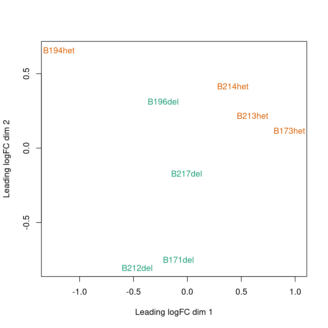
Figure 1: MDS plot coloured by genotype.

DE analysis

Fit a model with a term for genotype using the quasi-likelihood pipeline from edgeR.

Show code

y <- estimateDisp(y, y_design)
par(mfrow = c(1, 2))
plotBCV(y)
y_dgeglm <- glmQLFit(y, y_design, robust = TRUE)
plotQLDisp(y_dgeglm)

Show code

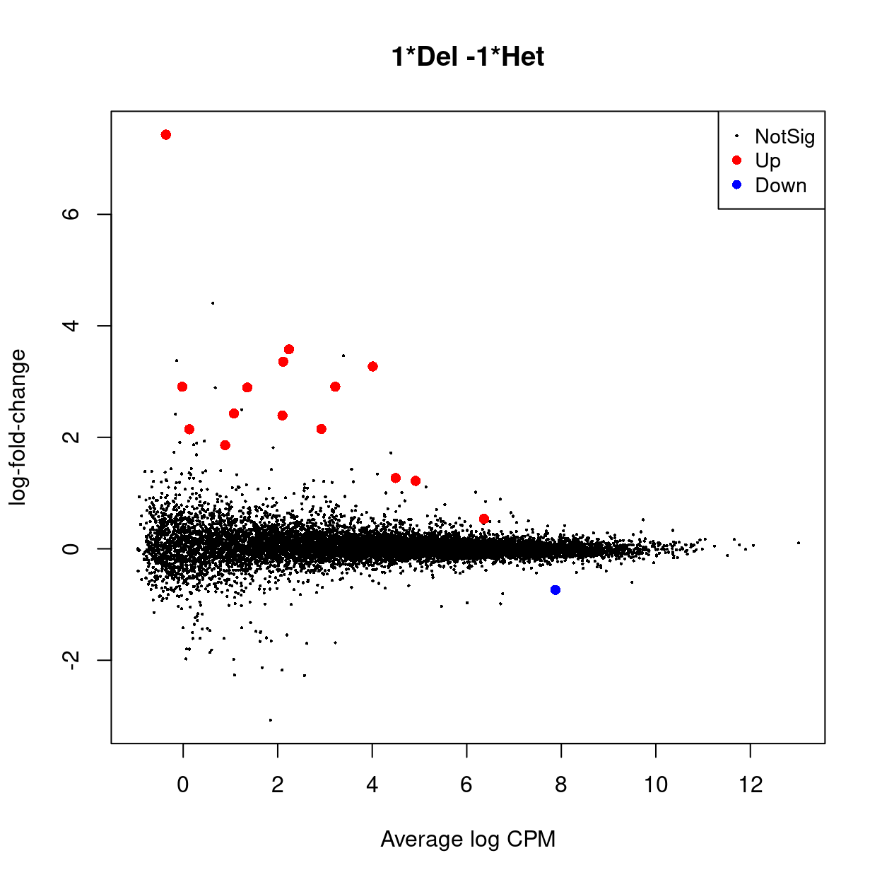
y_contrast <- makeContrasts(Del - Het, levels = y_design)
y_dgelrt <- glmQLFTest(y_dgeglm, contrast = y_contrast)
y_dt <- decideTests(y_dgelrt)

summary(y_dt) %>%
  knitr::kable(caption = "Number of DEGs (FDR < 0.05)")

Table 1: Number of DEGs (FDR < 0.05)

	1Del -1Het
Down	1
NotSig	13393
Up	15

CSV file of results available from output/DEGs/male_B_cells/.

Show code

gzout <- gzfile(
  description = file.path(outdir, "male_B_cells.DEGs.csv.gz"),
  open = "wb")
write.csv(
  topTags(y_dgelrt, n = Inf),
  gzout,
  # NOTE: quote = TRUE needed because some fields contain commas.
  quote = TRUE,
  row.names = FALSE)
close(gzout)

Show code

par(mfrow = c(1, 1))
plotMD(y_dgelrt)

Figure 2: MD plot highlighting DEGs (red).

An interactive Glimma MD plot of the differential expression results is available from output/DEGs/male_B_cells/glimma-plots/male_B_cells.md-plot.html.

Show code

glMDPlot(
  x = y_dgelrt,
  counts = y,
  anno = y$genes,
  display.columns = c("ENSEMBL.SYMBOL"),
  groups = y$samples$group,
  samples = colnames(y),
  status = y_dt,
  transform = TRUE,
  sample.cols = as.integer(factor(y$samples$genotype)),
  path = outdir,
  html = "male_B_cells.md-plot",
  launch = FALSE)

Gene set tests

Gene set testing is commonly used to interpret the differential expression results in a biological context. Here we apply various gene set tests to the DEG lists.

goana

We use the goana() function from the limma R/Bioconductor package to test for over-representation of gene ontology (GO) terms in each DEG list.

Show code

list_of_go <- lapply(colnames(y_contrast), function(j) {
  dgelrt <- glmLRT(y_dgeglm, contrast = y_contrast[, j])
  
  go <- goana(
    de = dgelrt,
    geneid = sapply(strsplit(dgelrt$genes$NCBI.ENTREZID, "; "), "[[", 1),
    species = "Mm")
  gzout <- gzfile(
    description = file.path(outdir, "male_B_cells.goana.csv.gz"),
    open = "wb")
  write.csv(
    topGO(go, number = Inf),
    gzout,
    row.names = TRUE)
  close(gzout)
  go
})
names(list_of_go) <- colnames(y_contrast)

CSV files of the results are available from output/DEGs/male_B_cells/.

An example of the results are shown below.

Show code

topGO(list_of_go[[1]]) %>%
  knitr::kable(
    caption = '`goana()` produces a table with a row for each GO term and the following columns: **Term** (GO term); **Ont** (ontology that the GO term belongs to. Possible values are "BP", "CC" and "MF"); **N** (number of genes in the GO term); **Up** (number of up-regulated differentially expressed genes); **Down** (number of down-regulated differentially expressed genes); **P.Up** (p-value for over-representation of GO term in up-regulated genes); **P.Down** (p-value for over-representation of GO term in down-regulated genes)')

Table 2: goana() produces a table with a row for each GO term and the following columns: Term (GO term); Ont (ontology that the GO term belongs to. Possible values are “BP,” “CC” and “MF”); N (number of genes in the GO term); Up (number of up-regulated differentially expressed genes); Down (number of down-regulated differentially expressed genes); P.Up (p-value for over-representation of GO term in up-regulated genes); P.Down (p-value for over-representation of GO term in down-regulated genes)

	Term	Ont	N	Up	Down	P.Up	P.Down
GO:0031720	haptoglobin binding	MF	4	0	4	1.0000000	0.0000000
GO:0005833	hemoglobin complex	CC	4	0	4	1.0000000	0.0000000
GO:0048731	system development	BP	2947	31	31	0.0131091	0.0000000
GO:0030426	growth cone	CC	164	1	10	0.6976242	0.0000000
GO:0030427	site of polarized growth	CC	170	1	10	0.7106582	0.0000000
GO:0031838	haptoglobin-hemoglobin complex	CC	5	1	4	0.0355835	0.0000000
GO:0007275	multicellular organism development	BP	3301	34	31	0.0121146	0.0000000
GO:0048821	erythrocyte development	BP	38	0	6	1.0000000	0.0000000
GO:0048468	cell development	BP	1486	16	21	0.0652232	0.0000000
GO:0007399	nervous system development	BP	1490	17	21	0.0364729	0.0000000
GO:0019825	oxygen binding	MF	8	0	4	1.0000000	0.0000000
GO:0150034	distal axon	CC	247	2	10	0.5353054	0.0000000
GO:0044297	cell body	CC	522	3	13	0.7331790	0.0000000
GO:0048856	anatomical structure development	BP	3597	36	31	0.0148414	0.0000000
GO:0032502	developmental process	BP	3893	36	32	0.0477809	0.0000000
GO:0005344	oxygen carrier activity	MF	3	0	3	1.0000000	0.0000000
GO:0048858	cell projection morphogenesis	BP	453	8	12	0.0164555	0.0000000
GO:0032501	multicellular organismal process	BP	4220	42	33	0.0077364	0.0000001
GO:0001944	vasculature development	BP	494	17	3	0.0000001	0.2635084
GO:0032990	cell part morphogenesis	BP	474	8	12	0.0209935	0.0000001

kegga

We use the kegga() function from the limma R/Bioconductor package to test for over-representation of KEGG pathways in each DEG list.

Show code

list_of_kegg <- lapply(colnames(y_contrast), function(j) {
  dgelrt <- glmLRT(y_dgeglm, contrast = y_contrast[, j])
  
  kegg <- kegga(
    de = dgelrt,
    geneid = sapply(strsplit(dgelrt$genes$NCBI.ENTREZID, "; "), "[[", 1),
    species = "Mm")
  gzout <- gzfile(
    description = file.path(outdir, "male_B_cells.kegga.csv.gz"),
    open = "wb")
  write.csv(
    topKEGG(kegg, number = Inf),
    gzout,
    row.names = TRUE)
  close(gzout)
  kegg
})
names(list_of_kegg) <- colnames(y_contrast)

CSV files of the results are available from output/DEGs/male_B_cells/.

An example of the results are shown below.

Show code

topKEGG(list_of_kegg[[1]]) %>%
  knitr::kable(
    caption = '`kegga()` produces a table with a row for each KEGG pathway ID and the following columns: **Pathway** (KEGG pathway); **N** (number of genes in the GO term); **Up** (number of up-regulated differentially expressed genes); **Down** (number of down-regulated differentially expressed genes); **P.Up** (p-value for over-representation of KEGG pathway in up-regulated genes); **P.Down** (p-value for over-representation of KEGG pathway in down-regulated genes)')

Table 3: kegga() produces a table with a row for each KEGG pathway ID and the following columns: Pathway (KEGG pathway); N (number of genes in the GO term); Up (number of up-regulated differentially expressed genes); Down (number of down-regulated differentially expressed genes); P.Up (p-value for over-representation of KEGG pathway in up-regulated genes); P.Down (p-value for over-representation of KEGG pathway in down-regulated genes)

	Pathway	N	Up	Down	P.Up	P.Down
path:mmu05143	African trypanosomiasis	26	1	4	0.1735812	0.0000021
path:mmu04668	TNF signaling pathway	92	7	0	0.0000046	1.0000000
path:mmu04380	Osteoclast differentiation	111	7	0	0.0000160	1.0000000
path:mmu05144	Malaria	46	1	4	0.2865069	0.0000216
path:mmu04657	IL-17 signaling pathway	57	5	0	0.0000576	1.0000000
path:mmu05418	Fluid shear stress and atherosclerosis	112	6	0	0.0001647	1.0000000
path:mmu01522	Endocrine resistance	78	5	0	0.0002573	1.0000000
path:mmu04915	Estrogen signaling pathway	79	5	1	0.0002731	0.2491464
path:mmu04935	Growth hormone synthesis, secretion and action	88	5	0	0.0004509	1.0000000
path:mmu05133	Pertussis	54	4	0	0.0006355	1.0000000
path:mmu04713	Circadian entrainment	57	4	0	0.0007807	1.0000000
path:mmu05224	Breast cancer	101	5	0	0.0008464	1.0000000
path:mmu05030	Cocaine addiction	30	3	0	0.0013240	1.0000000
path:mmu05200	Pathways in cancer	376	9	2	0.0016617	0.3953707
path:mmu04024	cAMP signaling pathway	118	5	0	0.0016969	1.0000000
path:mmu05135	Yersinia infection	123	5	0	0.0020368	1.0000000
path:mmu04620	Toll-like receptor signaling pathway	78	4	0	0.0025097	1.0000000
path:mmu05142	Chagas disease	83	4	0	0.0031451	1.0000000
path:mmu04670	Leukocyte transendothelial migration	83	4	0	0.0031451	1.0000000
path:mmu04926	Relaxin signaling pathway	86	4	0	0.0035748	1.0000000

camera with MSigDB gene sets

We use the camera() function from the limma R/Bioconductor package to test whether a set of genes is highly ranked relative to other genes in terms of differential expression, accounting for inter-gene correlation. Specifically, we test using gene sets from MSigDB, namely:

We download these gene sets from http://bioinf.wehi.edu.au/MSigDB/index.html

• H: hallmark gene sets are coherently expressed signatures derived by aggregating many MSigDB gene sets to represent well-defined biological states or processes.
• C2: curated gene sets from online pathway databases, publications in PubMed, and knowledge of domain experts.

Show code

# NOTE: Using BiocFileCache to avoid re-downloading these gene sets everytime 
#       the report is rendered.
library(BiocFileCache)
bfc <- BiocFileCache()
# NOTE: Creating list of gene sets in this slightly convoluted way so that each 
#       gene set name is prepended by its origin (e.g. H, C2, or C7).
msigdb <- do.call(
  c, 
  list(
    H = readRDS(
      bfcrpath(
        bfc,
        "http://bioinf.wehi.edu.au/MSigDB/v7.1/Mm.h.all.v7.1.entrez.rds")),
    C2 = readRDS(
      bfcrpath(
        bfc, 
        "http://bioinf.wehi.edu.au/MSigDB/v7.1/Mm.c2.all.v7.1.entrez.rds"))))

y_idx <- ids2indices(
  msigdb, 
  id = sapply(strsplit(y$genes$NCBI.ENTREZID, "; "), "[[", 1))
list_of_camera <- lapply(colnames(y_contrast), function(j) {
  cam <- camera(
    y = y, 
    index = y_idx,
    design = y_design, 
    contrast = y_contrast[, j])
  gzout <- gzfile(
    description = file.path(outdir, "male_B_cells.camera.csv.gz"),
    open = "wb")
  write.csv(
    cam,
    gzout,
    row.names = TRUE)
  close(gzout)
  cam
})
names(list_of_camera) <- colnames(y_contrast)

CSV files of the results are available from output/DEGs/male_B_cells.

An example of the results are shown below.

Show code

head(list_of_camera[[1]]) %>%
  knitr::kable(
    caption = '`camera()` produces a table with a row for each gene set (prepended by which MSigDB collection it comes from) and the following columns: **NGenes** (number of genes in set); **Direction** (direction of change); **PValue** (two-tailed p-value); **FDR** (Benjamini and Hochberg FDR adjusted p-value).')

Table 4: camera() produces a table with a row for each gene set (prepended by which MSigDB collection it comes from) and the following columns: NGenes (number of genes in set); Direction (direction of change); PValue (two-tailed p-value); FDR (Benjamini and Hochberg FDR adjusted p-value).

	NGenes	Direction	PValue	FDR
C2.ZHOU_PANCREATIC_EXOCRINE_PROGENITOR	3	Up	0	0e+00
C2.MORI_MATURE_B_LYMPHOCYTE_DN	92	Down	0	0e+00
C2.REACTOME_EUKARYOTIC_TRANSLATION_ELONGATION	108	Up	0	0e+00
C2.KEGG_RIBOSOME	103	Up	0	0e+00
C2.LEE_EARLY_T_LYMPHOCYTE_UP	116	Down	0	1e-07
C2.REACTOME_RESPONSE_OF_EIF2AK4_GCN2_TO_AMINO_ACID_DEFICIENCY	117	Up	0	2e-07

Sarah’s gene lists

Show code

y_X <- y$genes$ENSEMBL.SEQNAME == "X"

y_index <- list(`X-linked` = y_X)

Sarah requested testing all X-linked genes as a gene set.

We use the fry() function from the edgeR R/Bioconductor package to perform a self-contained gene set test against the null hypothesis that none of the genes in the set are differentially expressed.

Show code

fry(
  y,
  index = y_index,
  design = y_design,
  contrast = y_contrast, 
  sort = "none") %>%
    knitr::kable(
      caption = "Results of applying `fry()` to the RNA-seq differential expression results using the supplied gene sets. A significant 'Up' P-value means that the differential expression results found in the RNA-seq data are positively correlated with the expression signature from the corresponding gene set. Conversely, a significant 'Down' P-value means that the differential expression log-fold-changes are negatively correlated with the expression signature from the corresponding gene set. A significant 'Mixed' P-value means that the genes in the set tend to be differentially expressed without regard for direction.")

Table 5: Results of applying fry() to the RNA-seq differential expression results using the supplied gene sets. A significant ‘Up’ P-value means that the differential expression results found in the RNA-seq data are positively correlated with the expression signature from the corresponding gene set. Conversely, a significant ‘Down’ P-value means that the differential expression log-fold-changes are negatively correlated with the expression signature from the corresponding gene set. A significant ‘Mixed’ P-value means that the genes in the set tend to be differentially expressed without regard for direction.

	NGenes	Direction	PValue	PValue.Mixed
X-linked	416	Down	0.9861314	0.6496793

Show code

geneSetTestFiguresForPaper <- function() {
  for (n in names(y_index)) {
    if (is.data.frame(y_index[[n]])) {
      y_status <- rep(0, nrow(y_dgelrt))
      y_status[rownames(y) %in% y_index[[n]][, 1]] <-
        sign(y_index[[n]][y_index[[n]][, 1] %in% rownames(y), 2])
      plotMD(
        y_dgelrt,
        status = y_status,
        hl.col = c("red", "blue"),
        legend = "bottomright",
        main = n)
      abline(h = 0, col = "darkgrey")
    } else {
      y_status <- rep("Other", nrow(y_dgelrt))
      y_status[y_index[[n]]] <- n
      plotMD(
        y_dgelrt,
        status = y_status,
        values = n,
        hl.col = "red",
        legend = "topright",
        main = n)
      abline(h = 0, col = "darkgrey")
    }
    
    if (is.data.frame(y_index[[n]])) {
      barcodeplot(
        y_dgelrt$table$logFC,
        rownames(y) %in% y_index[[n]][, 1],
        gene.weights = y_index[[n]][
          y_index[[n]][, 1] %in% rownames(y), 2])
    } else {
      barcodeplot(
        y_dgelrt$table$logFC,
        y_index[[n]])
    }
  }
}

Show code

par(mfrow = c(length(y_index), 2))
geneSetTestFiguresForPaper()  

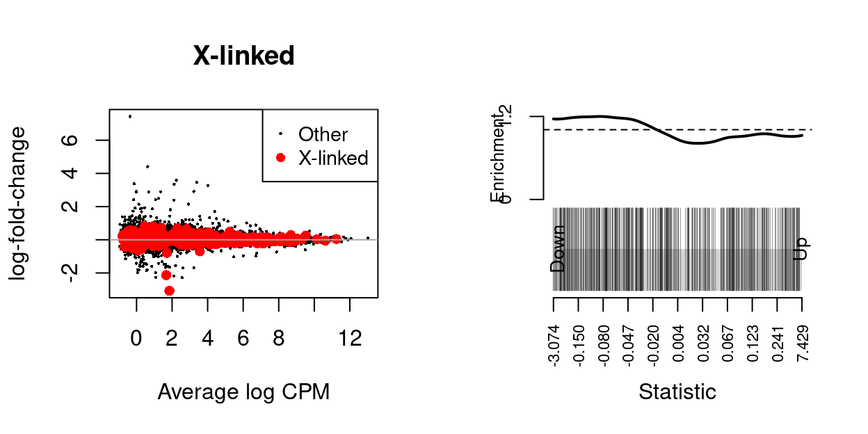
Figure 3: MD-plot and barcode plot of genes in supplied gene sets. Directional gene sets have (1) MD plot points coloured according to the statistical significance of the gene in the gene set (2) barcode plot ‘weights’ given by the logFC of the gene in the gene set. For the barcode plot, genes are represented by bars and are ranked from left to right by increasing log-fold change. This forms the barcode-like pattern. The line (or worm) above the barcode shows the relative local enrichment of the vertical bars in each part of the plot. The dotted horizontal line indicates neutral enrichment; the worm above the dotted line shows enrichment while the worm below the dotted line shows depletion.

A PDF version of these figures are available in output/figures/paper/male.gene_set_tests.pdf.

Show code

dir.create(here("output/figures/paper"))
pdf(
  here("output/figures/paper/male.gene_set_tests.pdf"),
  height = 6,
  width = 6)
par(mfrow = c(1, 1))
geneSetTestFiguresForPaper()
dev.off()

Session info

The analysis and this document were prepared using the following software (click triangle to expand)

Show code

sessioninfo::session_info()

─ Session info ─────────────────────────────────────────────────────
 setting  value                       
 version  R version 4.0.3 (2020-10-10)
 os       CentOS Linux 7 (Core)       
 system   x86_64, linux-gnu           
 ui       X11                         
 language (EN)                        
 collate  en_US.UTF-8                 
 ctype    en_US.UTF-8                 
 tz       Australia/Melbourne         
 date     2021-10-20                  

─ Packages ─────────────────────────────────────────────────────────
 ! package                            * version  date       lib
 P annotate                             1.68.0   2020-10-27 [?]
 P AnnotationDbi                      * 1.52.0   2020-10-27 [?]
 P AnnotationFilter                   * 1.14.0   2020-10-27 [?]
 P askpass                              1.1      2019-01-13 [?]
 P assertthat                           0.2.1    2019-03-21 [?]
 P beachmat                             2.6.4    2020-12-20 [?]
 P Biobase                            * 2.50.0   2020-10-27 [?]
 P BiocFileCache                      * 1.14.0   2020-10-27 [?]
 P BiocGenerics                       * 0.36.0   2020-10-27 [?]
 P BiocManager                          1.30.10  2019-11-16 [?]
 P BiocParallel                         1.24.1   2020-11-06 [?]
 P BiocStyle                            2.18.1   2020-11-24 [?]
 P biomaRt                              2.46.3   2021-02-09 [?]
 P Biostrings                           2.58.0   2020-10-27 [?]
 P bit                                  4.0.4    2020-08-04 [?]
 P bit64                                4.0.5    2020-08-30 [?]
 P bitops                               1.0-6    2013-08-17 [?]
 P blob                                 1.2.1    2020-01-20 [?]
 P cachem                               1.0.4    2021-02-13 [?]
 P cli                                  2.3.1    2021-02-23 [?]
 P colorspace                           2.0-0    2020-11-11 [?]
 P crayon                               1.4.1    2021-02-08 [?]
 P crosstalk                            1.1.1    2021-01-12 [?]
 P curl                                 4.3      2019-12-02 [?]
 P data.table                           1.14.0   2021-02-21 [?]
 P DBI                                  1.1.1    2021-01-15 [?]
 P dbplyr                             * 2.1.0    2021-02-03 [?]
 P DelayedArray                         0.16.1   2021-01-22 [?]
 P DelayedMatrixStats                   1.12.3   2021-02-03 [?]
 P DESeq2                               1.30.1   2021-02-19 [?]
 P digest                               0.6.27   2020-10-24 [?]
 P distill                              1.2      2021-01-13 [?]
 P downlit                              0.2.1    2020-11-04 [?]
 P dplyr                                1.0.4    2021-02-02 [?]
 P DT                                   0.17     2021-01-06 [?]
 P edgeR                              * 3.32.1   2021-01-14 [?]
 P ellipsis                             0.3.1    2020-05-15 [?]
 P EnsDb.Mmusculus.v79                * 2.99.0   2020-07-15 [?]
 P ensembldb                          * 2.14.0   2020-10-27 [?]
 P evaluate                             0.14     2019-05-28 [?]
 P fansi                                0.4.2    2021-01-15 [?]
 P fastmap                              1.1.0    2021-01-25 [?]
 P genefilter                           1.72.1   2021-01-21 [?]
 P geneplotter                          1.68.0   2020-10-27 [?]
 P generics                             0.1.0    2020-10-31 [?]
 P GenomeInfoDb                       * 1.26.2   2020-12-08 [?]
 P GenomeInfoDbData                     1.2.4    2020-10-20 [?]
 P GenomicAlignments                    1.26.0   2020-10-27 [?]
 P GenomicFeatures                    * 1.42.1   2020-11-12 [?]
 P GenomicRanges                      * 1.42.0   2020-10-27 [?]
 P ggplot2                              3.3.3    2020-12-30 [?]
 P Glimma                             * 2.0.0    2020-10-27 [?]
 P glue                                 1.4.2    2020-08-27 [?]
 P GO.db                              * 3.12.1   2020-11-04 [?]
 P graph                                1.68.0   2020-10-27 [?]
 P gtable                               0.3.0    2019-03-25 [?]
 P here                               * 1.0.1    2020-12-13 [?]
 P highr                                0.8      2019-03-20 [?]
 P hms                                  1.0.0    2021-01-13 [?]
 P htmltools                            0.5.1.1  2021-01-22 [?]
 P htmlwidgets                          1.5.3    2020-12-10 [?]
 P httr                                 1.4.2    2020-07-20 [?]
 P IRanges                            * 2.24.1   2020-12-12 [?]
 P jsonlite                             1.7.2    2020-12-09 [?]
 P knitr                                1.31     2021-01-27 [?]
 P lattice                              0.20-41  2020-04-02 [3]
 P lazyeval                             0.2.2    2019-03-15 [?]
 P lifecycle                            1.0.0    2021-02-15 [?]
 P limma                              * 3.46.0   2020-10-27 [?]
 P locfit                               1.5-9.4  2020-03-25 [?]
 P magrittr                             2.0.1    2020-11-17 [?]
 P Matrix                               1.2-18   2019-11-27 [3]
 P MatrixGenerics                       1.2.1    2021-01-30 [?]
 P matrixStats                          0.58.0   2021-01-29 [?]
 P memoise                              2.0.0    2021-01-26 [?]
 P msigdbr                            * 7.2.1    2020-10-02 [?]
 P munsell                              0.5.0    2018-06-12 [?]
 P Mus.musculus                       * 1.3.1    2020-07-15 [?]
 P openssl                              1.4.3    2020-09-18 [?]
 P org.Mm.eg.db                       * 3.12.0   2020-10-20 [?]
 P OrganismDbi                        * 1.32.0   2020-10-27 [?]
 P pillar                               1.5.0    2021-02-22 [?]
 P pkgconfig                            2.0.3    2019-09-22 [?]
 P prettyunits                          1.1.1    2020-01-24 [?]
 P progress                             1.2.2    2019-05-16 [?]
 P ProtGenerics                         1.22.0   2020-10-27 [?]
 P purrr                                0.3.4    2020-04-17 [?]
 P R6                                   2.5.0    2020-10-28 [?]
 P rappdirs                             0.3.3    2021-01-31 [?]
 P RBGL                                 1.66.0   2020-10-27 [?]
 P RColorBrewer                         1.1-2    2014-12-07 [?]
 P Rcpp                                 1.0.6    2021-01-15 [?]
 P RCurl                                1.98-1.2 2020-04-18 [?]
 P rlang                                0.4.10   2020-12-30 [?]
 P rmarkdown                            2.11     2021-09-14 [?]
 P rprojroot                            2.0.2    2020-11-15 [?]
 P Rsamtools                            2.6.0    2020-10-27 [?]
 P RSQLite                              2.2.3    2021-01-24 [?]
 P rtracklayer                          1.50.0   2020-10-27 [?]
 P S4Vectors                          * 0.28.1   2020-12-09 [?]
 P scales                             * 1.1.1    2020-05-11 [?]
 P scuttle                              1.0.4    2020-12-17 [?]
 P sessioninfo                          1.1.1    2018-11-05 [?]
 P SingleCellExperiment                 1.12.0   2020-10-27 [?]
 P sparseMatrixStats                    1.2.1    2021-02-02 [?]
 P statmod                              1.4.35   2020-10-19 [?]
 P stringi                              1.5.3    2020-09-09 [?]
 P stringr                              1.4.0    2019-02-10 [?]
 P SummarizedExperiment                 1.20.0   2020-10-27 [?]
 P survival                             3.2-7    2020-09-28 [3]
 P tibble                               3.0.6    2021-01-29 [?]
 P tidyselect                           1.1.0    2020-05-11 [?]
 P TxDb.Mmusculus.UCSC.mm10.knownGene * 3.10.0   2020-07-15 [?]
 P utf8                                 1.1.4    2018-05-24 [?]
 P vctrs                                0.3.6    2020-12-17 [?]
 P withr                                2.4.1    2021-01-26 [?]
 P xfun                                 0.26     2021-09-14 [?]
 P XML                                  3.99-0.5 2020-07-23 [?]
 P xml2                                 1.3.2    2020-04-23 [?]
 P xtable                               1.8-4    2019-04-21 [?]
 P XVector                              0.30.0   2020-10-27 [?]
 P yaml                                 2.2.1    2020-02-01 [?]
 P zlibbioc                             1.36.0   2020-10-27 [?]
 source        
 Bioconductor  
 Bioconductor  
 Bioconductor  
 CRAN (R 4.0.0)
 CRAN (R 4.0.0)
 Bioconductor  
 Bioconductor  
 Bioconductor  
 Bioconductor  
 CRAN (R 4.0.0)
 Bioconductor  
 Bioconductor  
 Bioconductor  
 Bioconductor  
 CRAN (R 4.0.0)
 CRAN (R 4.0.0)
 CRAN (R 4.0.0)
 CRAN (R 4.0.0)
 CRAN (R 4.0.3)
 CRAN (R 4.0.3)
 CRAN (R 4.0.3)
 CRAN (R 4.0.3)
 CRAN (R 4.0.3)
 CRAN (R 4.0.0)
 CRAN (R 4.0.3)
 CRAN (R 4.0.3)
 CRAN (R 4.0.3)
 Bioconductor  
 Bioconductor  
 Bioconductor  
 CRAN (R 4.0.2)
 CRAN (R 4.0.3)
 CRAN (R 4.0.3)
 CRAN (R 4.0.3)
 CRAN (R 4.0.3)
 Bioconductor  
 CRAN (R 4.0.0)
 Bioconductor  
 Bioconductor  
 CRAN (R 4.0.0)
 CRAN (R 4.0.3)
 CRAN (R 4.0.3)
 Bioconductor  
 Bioconductor  
 CRAN (R 4.0.3)
 Bioconductor  
 Bioconductor  
 Bioconductor  
 Bioconductor  
 Bioconductor  
 CRAN (R 4.0.3)
 Bioconductor  
 CRAN (R 4.0.0)
 Bioconductor  
 Bioconductor  
 CRAN (R 4.0.0)
 CRAN (R 4.0.3)
 CRAN (R 4.0.0)
 CRAN (R 4.0.3)
 CRAN (R 4.0.3)
 CRAN (R 4.0.3)
 CRAN (R 4.0.0)
 Bioconductor  
 CRAN (R 4.0.3)
 CRAN (R 4.0.3)
 CRAN (R 4.0.3)
 CRAN (R 4.0.0)
 CRAN (R 4.0.3)
 Bioconductor  
 CRAN (R 4.0.0)
 CRAN (R 4.0.3)
 CRAN (R 4.0.3)
 Bioconductor  
 CRAN (R 4.0.3)
 CRAN (R 4.0.3)
 CRAN (R 4.0.2)
 CRAN (R 4.0.0)
 Bioconductor  
 CRAN (R 4.0.2)
 Bioconductor  
 Bioconductor  
 CRAN (R 4.0.3)
 CRAN (R 4.0.0)
 CRAN (R 4.0.0)
 CRAN (R 4.0.0)
 Bioconductor  
 CRAN (R 4.0.0)
 CRAN (R 4.0.2)
 CRAN (R 4.0.3)
 Bioconductor  
 CRAN (R 4.0.0)
 CRAN (R 4.0.3)
 CRAN (R 4.0.0)
 CRAN (R 4.0.3)
 CRAN (R 4.0.0)
 CRAN (R 4.0.3)
 Bioconductor  
 CRAN (R 4.0.3)
 Bioconductor  
 Bioconductor  
 CRAN (R 4.0.0)
 Bioconductor  
 CRAN (R 4.0.0)
 Bioconductor  
 Bioconductor  
 CRAN (R 4.0.2)
 CRAN (R 4.0.0)
 CRAN (R 4.0.0)
 Bioconductor  
 CRAN (R 4.0.3)
 CRAN (R 4.0.3)
 CRAN (R 4.0.0)
 Bioconductor  
 CRAN (R 4.0.0)
 CRAN (R 4.0.3)
 CRAN (R 4.0.3)
 CRAN (R 4.0.0)
 CRAN (R 4.0.0)
 CRAN (R 4.0.0)
 CRAN (R 4.0.0)
 Bioconductor  
 CRAN (R 4.0.0)
 Bioconductor  

[1] /stornext/Projects/score/Analyses/C086_Kinkel/renv/library/R-4.0/x86_64-pc-linux-gnu
[2] /tmp/RtmpfgojZ6/renv-system-library
[3] /stornext/System/data/apps/R/R-4.0.3/lib64/R/library

 P ── Loaded and on-disk path mismatch.

---

1. Ensembl gene ID↩︎

2. Some care is taken to account for missing and duplicate gene symbols; missing symbols are replaced with the Ensembl identifier and duplicated symbols are concatenated with the (unique) Ensembl identifiers.↩︎