Multi-sample comparisons of the Kinkel (C086) Smchd1 LSK mini-bulk data set

Read-based analysis

Summary

This report analyses the read counts of the Del and Het samples only. The report begins with some general Setup and is followed by various analyses denoted by a prefix (y, ym, yf):

• y: Analysis of aggregated technical replicates with Remove Unwanted Variation (RUV) normalization
• ym: Male-only: analysis of aggregated technical replicates using RUV normalization
• yf: Female-only: analysis of aggregated technical replicates using RUV normalization

Setup

Show code

library(SingleCellExperiment)
library(here)
library(edgeR)
library(ggplot2)
library(cowplot)
library(patchwork)
library(ggrepel)
library(magrittr)
library(Glimma)
library(EDASeq)
library(RUVSeq)
library(pheatmap)

source(here("code/helper_functions.R"))

Load data

Show code

sce <- readRDS(here("data", "SCEs", "C086_Kinkel.preprocessed.SCE.rds"))
# NOTE: Reorder samples for plots (e.g., RLE plots).
sce <- sce[, order(sce$smchd1_genotype_updated, sce$sex, sce$mouse_number)]

# Restrict analysis to read counts
assays(sce) <- list(counts = assay(sce, "read_counts"))

outdir <- here("output", "DEGs", "reads")
dir.create(outdir, recursive = TRUE)

Gene filtering

We filter the genes to only retain protein coding genes.

Show code

sce <- sce[any(grepl("protein_coding", rowData(sce)$ENSEMBL.GENEBIOTYPE)), ]

Sample filtering

We filter out the WT samples as these are not useful for DE analysis since there is only 1 biological replicate.

Show code

sce <- sce[, sce$smchd1_genotype_updated != "WT"]

Show code

colData(sce) <- droplevels(colData(sce))
# Some useful colours
sex_colours <- setNames(
  unique(sce$sex_colours),
  unique(names(sce$sex_colours)))
smchd1_genotype_updated_colours <- setNames(
  unique(sce$smchd1_genotype_updated_colours),
  unique(names(sce$smchd1_genotype_updated_colours)))
mouse_number_colours <- setNames(
  unique(sce$mouse_number_colours),
  unique(names(sce$mouse_number_colours)))

Create DGEList objects

Show code

x <- DGEList(
  counts = as.matrix(counts(sce)),
  samples = colData(sce),
  group = factor(sce$smchd1_genotype_updated),
  genes = flattenDF(rowData(sce)))
x <- x[rowSums(x$counts) > 0, ]

Show code

y <- sumTechReps(x, x$samples$genotype.mouse)
ym <- y[, y$samples$sex == "M"]
yf <- y[, y$samples$sex == "F"]

Gene filtering

For each analysis, shown are the number of genes that have sufficient counts to test for DE (TRUE) or not (FALSE).

y

Show code

y_keep_exprs <- filterByExpr(y, group = y$samples$group, min.count = 5)
y <- y[y_keep_exprs, , keep.lib.sizes = FALSE]
table(y_keep_exprs)

y_keep_exprs
FALSE  TRUE 
 3040 11450 

ym

Show code

ym_keep_exprs <- filterByExpr(ym, group = ym$samples$group, min.count = 5)
ym <- ym[ym_keep_exprs, , keep.lib.sizes = FALSE]
table(ym_keep_exprs)

ym_keep_exprs
FALSE  TRUE 
 2891 11599 

yf

Show code

yf_keep_exprs <- filterByExpr(yf, group = yf$samples$group, min.count = 5)
yf <- yf[yf_keep_exprs, , keep.lib.sizes = FALSE]
table(yf_keep_exprs)

yf_keep_exprs
FALSE  TRUE 
 2977 11513 

Normalization

Normalization with upper-quartile (UQ) normalization.

Show code

x <- calcNormFactors(x, method = "upperquartile")
y <- calcNormFactors(y, method = "upperquartile")
ym <- calcNormFactors(ym, method = "upperquartile")
yf <- calcNormFactors(yf, method = "upperquartile")

Aggregation of technical replicates

We have up to 3 technical replicates from each biological replicate. Ideally, the technical replicates are very similar to one another when view on an MDS plot. However, Figure 1 shows that:

• Some of the technical replicates are more variable than we would like
• Those ‘outlier’ samples have smaller library sizes

Show code

x_mds <- plotMDS(x, plot = FALSE)

x_df <- cbind(data.frame(x = x_mds$x, y = x_mds$y), x$samples)
rownames(x_df) <- colnames(x)

p1 <- ggplot(
  aes(x = x, y = y, colour = smchd1_genotype_updated, label = rownames(x_df)),
  data = x_df) +
  geom_point() +
  geom_text_repel(size = 2) +
  theme_cowplot(font_size = 8) +
  xlab("Leading logFC dim 1") +
  ylab("Leading logFC dim 2") +
  scale_colour_manual(values = smchd1_genotype_updated_colours)
p2 <- ggplot(
  aes(x = x, y = y, colour = sex, label = rownames(x_df)),
  data = x_df) +
  geom_point() +
  geom_text_repel(size = 2) +
  theme_cowplot(font_size = 8) +
  xlab("Leading logFC dim 1") +
  ylab("Leading logFC dim 2") +
  scale_colour_manual(values = sex_colours)
p3 <- ggplot(
  aes(x = x, y = y, colour = mouse_number, label = rownames(x_df)),
  data = x_df) +
  geom_point() +
  geom_text_repel(size = 2) +
  theme_cowplot(font_size = 8) +
  xlab("Leading logFC dim 1") +
  ylab("Leading logFC dim 2") +
  scale_colour_manual(values = mouse_number_colours)
p4 <- ggplot(
  aes(x = x, y = y, colour = log10(lib.size), label = rownames(x_df)),
  data = x_df) +
  geom_point() +
  geom_text_repel(size = 2) +
  theme_cowplot(font_size = 8) +
  scale_colour_viridis_c() +
  xlab("Leading logFC dim 1") +
  ylab("Leading logFC dim 2")

p1 + p2 + p3 + p4 + plot_layout(ncol = 2)

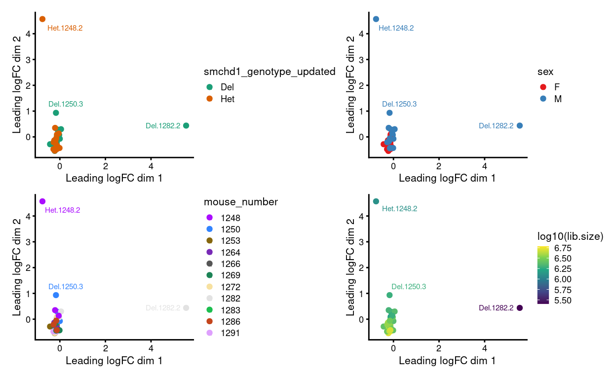
Figure 1: MDS plots of individual technical replicates coloured by various experimental factors.

Although we could analyse the data at the level of technical replicates, this is more complicated. It will make our life easier by aggregating these technical replicates so that we have 1 sample per biological replicate. To aggregate technical replicates we simply sum their counts.

Figure 2 shows the MDS plot after aggregating the technical replicates. We still observe that:

• Samples cluster more strongly by sex than by genotype
• Some of the variation is associated with library size

These observations (and others) prompt us to consider further normalization of the data.

Show code

y_mds <- plotMDS(y, plot = FALSE)

y_df <- cbind(data.frame(x = y_mds$x, y = y_mds$y), y$samples)
rownames(y_df) <- colnames(y)

p1 <- ggplot(
  aes(x = x, y = y, colour = smchd1_genotype_updated, label = rownames(y_df)),
  data = y_df) +
  geom_point() +
  geom_text_repel(size = 2) +
  theme_cowplot(font_size = 8) +
  xlab("Leading logFC dim 1") +
  ylab("Leading logFC dim 2") +
  scale_colour_manual(values = smchd1_genotype_updated_colours)
p2 <- ggplot(
  aes(x = x, y = y, colour = sex, label = rownames(y_df)),
  data = y_df) +
  geom_point() +
  geom_text_repel(size = 2) +
  theme_cowplot(font_size = 8) +
  xlab("Leading logFC dim 1") +
  ylab("Leading logFC dim 2") +
  scale_colour_manual(values = sex_colours)
p3 <- ggplot(
  aes(x = x, y = y, colour = mouse_number, label = rownames(y_df)),
  data = y_df) +
  geom_point() +
  geom_text_repel(size = 2) +
  theme_cowplot(font_size = 8) +
  xlab("Leading logFC dim 1") +
  ylab("Leading logFC dim 2") +
  scale_colour_manual(values = mouse_number_colours)
p4 <- ggplot(
  aes(x = x, y = y, colour = log10(lib.size), label = rownames(y_df)),
  data = y_df) +
  geom_point() +
  geom_text_repel(size = 2) +
  theme_cowplot(font_size = 8) +
  scale_colour_viridis_c() +
  xlab("Leading logFC dim 1") +
  ylab("Leading logFC dim 2")

p1 + p2 + p3 + p4 + plot_layout(ncol = 2)

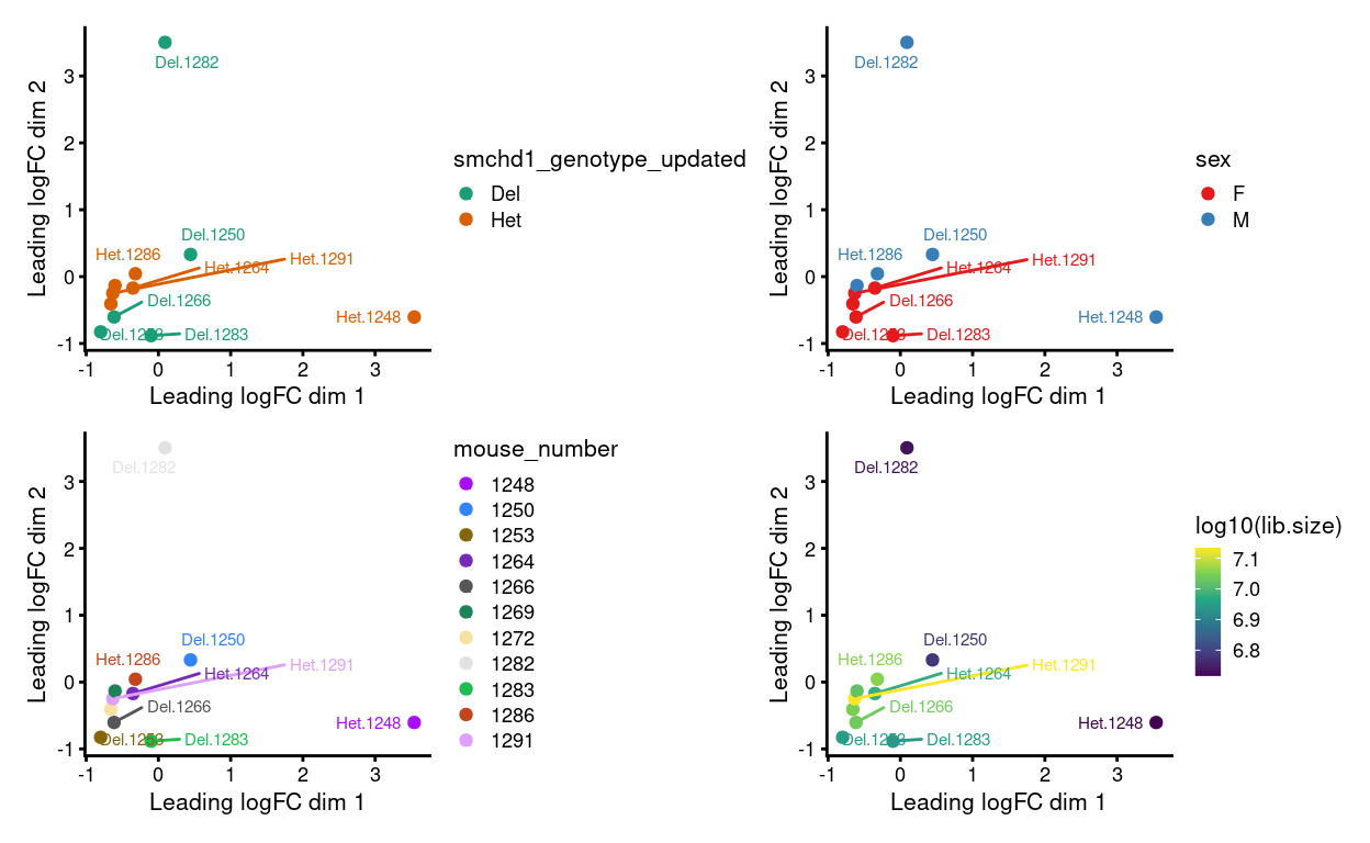
Figure 2: MDS plots of aggregated technical replicates coloured by various experimental factors.

Further normalization

Show code

design <- model.matrix(
  ~0 + smchd1_genotype_updated + sex,
  y$samples)
colnames(design) <- sub(
  "smchd1_genotype_updated|sex",
  "",
  colnames(design))

y <- estimateDisp(y, design)

dgeglm <- glmFit(y, design)
contrasts <- makeContrasts(Del - Het, levels = design)
dgelrt <- glmLRT(dgeglm, contrast = contrasts)
tt <- topTags(dgelrt, n = Inf)
summary(decideTests(dgelrt))

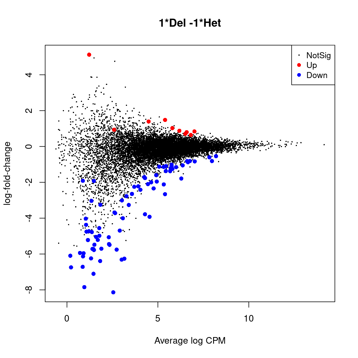
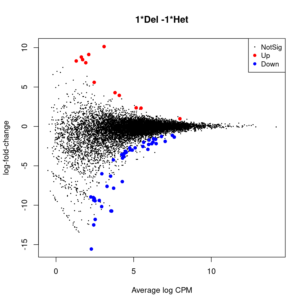
The MDS plots in Figure 2 strongly suggest that we will not detect many differentially expressed genes (DEGs) using a standard analysis. This is borne out in Figure 3, which shows the results of a standard edgeR analysis of the data (there is 3 DEG (\(FDR < 0.05\))).

Show code

par(mfrow = c(1, 2))
plotMD(dgelrt)
abline(h = 0, lty = 2, col = "dodgerBlue")
plotMD(
  dgelrt,
  status = ifelse(rownames(dgelrt) == "Smchd1", "Smchd1", "Other"),
  hl.col = "orange")
abline(h = 0, lty = 2, col = "dodgerBlue")

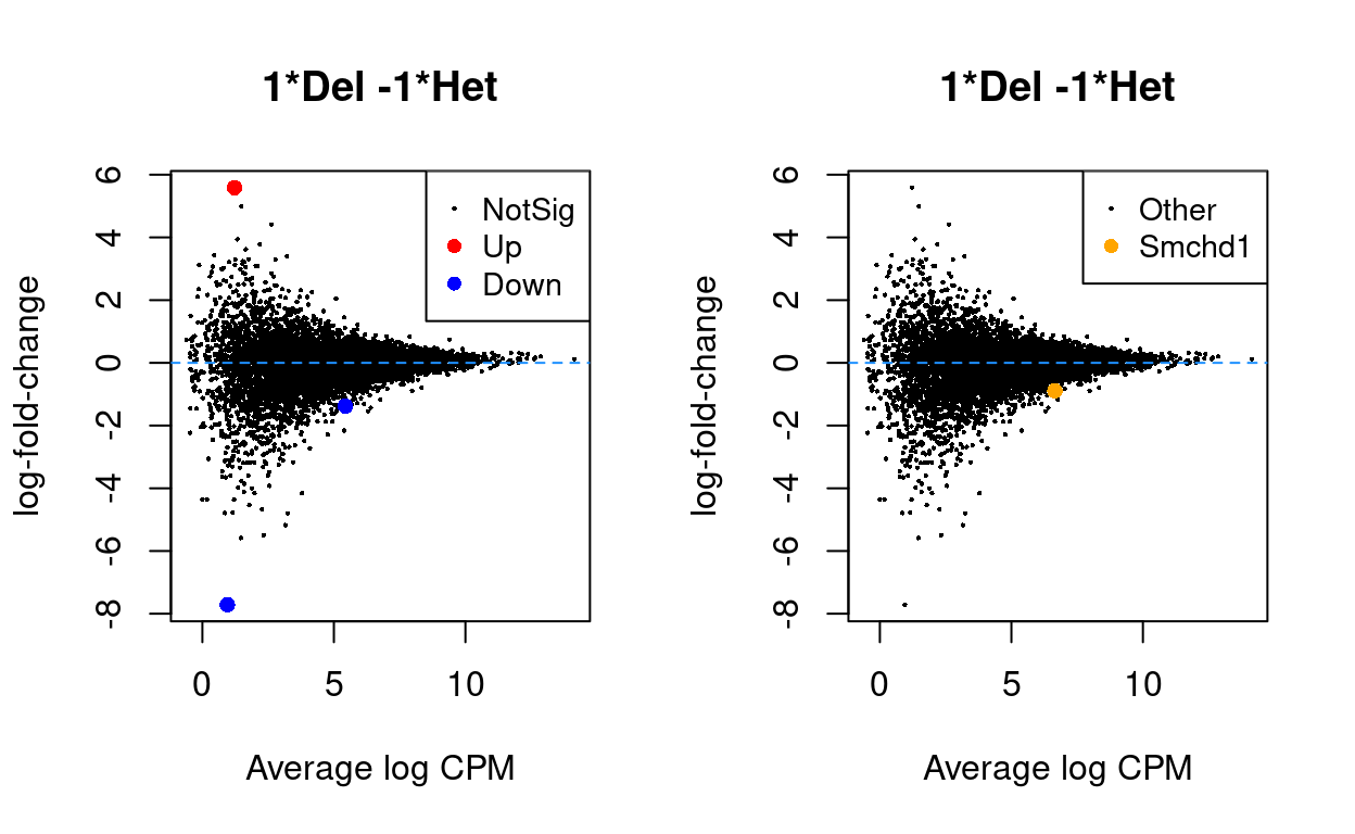
Figure 3: MD plot highlighting DE genes (left) and Smchd1 (right).

To further normalize the data, we use RUVs.

Show code

differences <- makeGroups(
  interaction(y$samples$smchd1_genotype_updated, y$samples$sex))
ruv <- RUVs(
    x = betweenLaneNormalization(y$counts, "upper"),
    cIdx = rownames(y),
    k = 3,
    scIdx = differences)

design <- model.matrix(
  ~0 + smchd1_genotype_updated + sex + ruv$W,
  y$samples)
colnames(design) <- sub(
  "ruv\\$|smchd1_genotype_updated|sex",
  "",
  colnames(design))

Figure 4 shows that after applying RUVs samples cluster by combination of genotype and sex, which is what we want to see.

Therefore, we opt to further normalize the data using RUVs in each DE analysis¹

Show code

y_mds <- plotMDS(cpm(ruv$normalizedCounts, log = TRUE), plot = FALSE)

y_df <- cbind(data.frame(x = y_mds$x, y = y_mds$y), y$samples)
rownames(y_df) <- colnames(y)

p1 <- ggplot(
  aes(x = x, y = y, colour = smchd1_genotype_updated, label = rownames(y_df)),
  data = y_df) +
  geom_point() +
  geom_text_repel(size = 2) +
  theme_cowplot(font_size = 8) +
  xlab("Leading logFC dim 1") +
  ylab("Leading logFC dim 2") +
  scale_colour_manual(values = smchd1_genotype_updated_colours)
p2 <- ggplot(
  aes(x = x, y = y, colour = sex, label = rownames(y_df)),
  data = y_df) +
  geom_point() +
  geom_text_repel(size = 2) +
  theme_cowplot(font_size = 8) +
  xlab("Leading logFC dim 1") +
  ylab("Leading logFC dim 2") +
  scale_colour_manual(values = sex_colours)
p3 <- ggplot(
  aes(x = x, y = y, colour = mouse_number, label = rownames(y_df)),
  data = y_df) +
  geom_point() +
  geom_text_repel(size = 2) +
  theme_cowplot(font_size = 8) +
  xlab("Leading logFC dim 1") +
  ylab("Leading logFC dim 2") +
  scale_colour_manual(values = mouse_number_colours)
p4 <- ggplot(
  aes(x = x, y = y, colour = log10(lib.size), label = rownames(y_df)),
  data = y_df) +
  geom_point() +
  geom_text_repel(size = 2) +
  theme_cowplot(font_size = 8) +
  scale_colour_viridis_c() +
  xlab("Leading logFC dim 1") +
  ylab("Leading logFC dim 2")

p1 + p2 + p3 + p4 + plot_layout(ncol = 2)

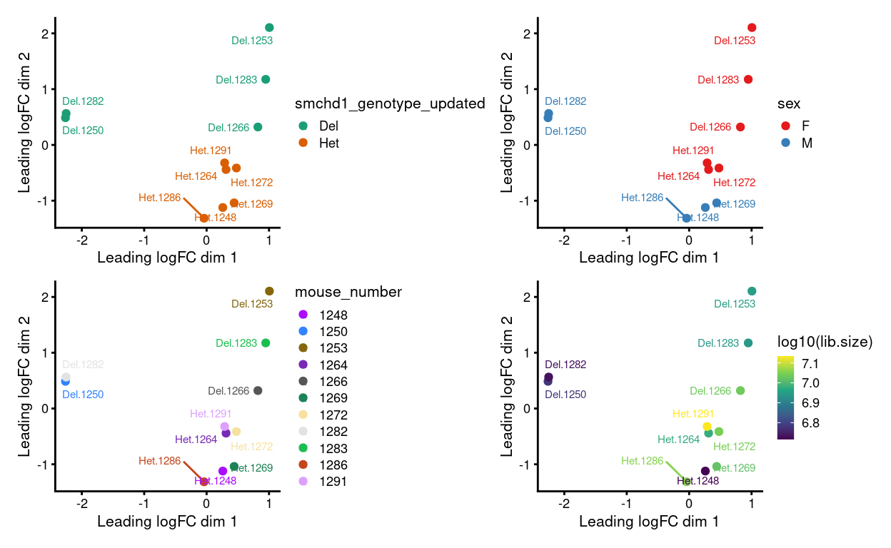
Figure 4: MDS plots of aggregated technical replicates following RUV coloured by various experimental factors.

Gene sets

Marnie and Sarah interested in the following gene sets:

These are available as Excel files in data/sarahs_gene_lists/. These genes are matched to the present dataset using the supplied gene symbol.

• Non-directional gene sets (i.e. no logFC available from previous data)
  • X-linked: Anything with ENSEMBL.SEQNAME set as ‘X’).
  • Protocadherin: Genes with symbol of the form Pcdh#.
  • Prader-Willi: Imprinted genes from the Prader-Willi cluster (Ndn, Mkrn3, Peg12)
  • Proliferation Group Venezia (2004): Genes that have their maximum expression at peak-cycling times (Time Of Max = TOM = 2, 3, and 6 days post-treatment) in a time-course experiment designed to stimulate adult HSCs to proliferate (Venezia et al. 2004).
    • The p-value (ANOVA) is based on about 1500 genes that changed significantly over the time course while the logFC is a separate comparison between FL HSCs (naturally proliferative) and adult HSCs (naturally quiescent).
    • We treat this as a non-directional gene set by ignoring the logFC because the specific comparison is not of interest.
  • Quiescence Group Venezia (2004): Genes that have their maximum expression at non-cycling times (Time Of Max = TOM = 0, 1, 10, and 30 days post-treatment) in a time-course experiment designed to stimulate adult HSCs to proliferate (Venezia et al. 2004).
    • The p-value (ANOVA) is based on about 1500 genes that changed significantly over the time course while the logFC is a separate comparison between FL HSCs (naturally proliferative) and adult HSCs (naturally quiescent).
    • We treat this as a non-directional gene set by ignoring the logFC because the specific comparison is not of interest.
• Directional gene sets (i.e. logFC available from previous data).
  • Male: Het vs. Del: DEGs from a comparison of male Smchd1-het and Smchd1-del B cells from aged mice (>12 months old)².
  • Female: Het vs. Del: DEGs from a comparison of female Smchd1-het and Smchd1-del B cells from aged mice (>12 months old)³.
  • Sun (2014): DEGs from a comparison of HSCs from young (2mo) and aged (24mo) male mice (Sun et al. 2014).
  • Chambers (2007): Upregulated DEGs from a comparison of HSCs to an average of all other cell types analysed (Chambers et al. 2007).
  • Gazit (2013): Genes with “enriched expression in HSCs”⁴ compared with all other hematopoietic cell types (Gazit et al. 2013).
    • Although no logFC is available, by definition these genes have a logFC > 0.
  • Chambers (2007) & Gazit (2013): The union of Chambers (2007) and Gazit (2013) with the logFC preferentially taken from Chambers (2007).
    • This is in the spirit of Vizán et al. (2020) who do a gene set enrichment analysis using “a merge of differentially expressed genes provided by Gazit (2013) and Chambers (2007)” but do not explain how they ‘merge’ these gene lists.

Show code

male_het_vs_del <- read.csv(
  here("output", "DEGs", "male_B_cells", "male_B_cells.DEGs.csv.gz"))
female_het_vs_del <- read.csv(
  here("output", "DEGs", "female_B_cells", "female_B_cells.DEGs.csv.gz"))
# NOTE: The `as.data.frame()` calls are needed because read_excel() returns a 
#       tibble but `limma::fry()` does not support tibbles.
library(readxl)
sun_2014 <- read_excel(
  here("data", "sarahs_gene_lists", "Sun_2014_CellStemCell_DE_HSC_aging.xlsx"),
  sheet = "Differentially expressed genes")
sun_2014 <- as.data.frame(sun_2014)
chambers_2007 <- read_excel(
  here("data", "sarahs_gene_lists", "HSC_signature_genes.xlsx"),
  sheet = "Chambers_2007_CellStemCell",
  na = "NA")
chambers_2007 <- as.data.frame(chambers_2007)
gazit_2013 <- read_excel(
  here("data", "sarahs_gene_lists", "HSC_signature_genes.xlsx"),
  sheet = "Gazit_2013_StemCellRep",
  range = "A3:C325")
gazit_2013 <- as.data.frame(gazit_2013)
# NOTE: File manually downloaded from   
#       https://doi.org/10.1371/journal.pbio.0020301.st002 and converted to a 
#       CSV file using LibreOffice.
venezia_proliferation <- read.csv(
  here("data", "sarahs_gene_lists", "pbio.0020301.st002.csv"),
  header = TRUE,
  skip = 1,
  nrow = 680)
# NOTE: File manually downloaded from   
#       https://doi.org/10.1371/journal.pbio.0020301.st004 and converted to a 
#       CSV file using LibreOffice.
venezia_quiescence <- read.csv(
  here("data", "sarahs_gene_lists", "pbio.0020301.st004.csv"),
  header = TRUE,
  skip = 1,
  nrow = 808)
smchd1_femBcells <- data.table::fread(
  here("data", "sarahs_gene_lists", "210923_EdgeR stats p1.0 log2.txt"),
  data.table = FALSE)

Analysis of aggregated technical replicates

Show code

y_differences <- makeGroups(
  interaction(y$samples$smchd1_genotype_updated, y$samples$sex))
y_ruv <- RUVs(
    x = betweenLaneNormalization(y$counts, "upper"),
    cIdx = rownames(y),
    k = 3,
    scIdx = y_differences)

y_design <- model.matrix(
  ~0 + smchd1_genotype_updated + sex + y_ruv$W,
  y$samples)
colnames(y_design) <- sub(
  "ruv\\$|smchd1_genotype_updated|sex",
  "",
  colnames(y_design))

MDS

Show code

y_mds <- plotMDS(cpm(y_ruv$normalizedCounts, log = TRUE), plot = FALSE)

y_df <- cbind(data.frame(x = y_mds$x, y = y_mds$y), y$samples)
rownames(y_df) <- colnames(y)

p1 <- ggplot(
  aes(x = x, y = y, colour = smchd1_genotype_updated, label = rownames(y_df)),
  data = y_df) +
  geom_point() +
  geom_text_repel(size = 2) +
  theme_cowplot(font_size = 8) +
  xlab("Leading logFC dim 1") +
  ylab("Leading logFC dim 2") +
  scale_colour_manual(values = smchd1_genotype_updated_colours)
p2 <- ggplot(
  aes(x = x, y = y, colour = sex, label = rownames(y_df)),
  data = y_df) +
  geom_point() +
  geom_text_repel(size = 2) +
  theme_cowplot(font_size = 8) +
  xlab("Leading logFC dim 1") +
  ylab("Leading logFC dim 2") +
  scale_colour_manual(values = sex_colours)
p3 <- ggplot(
  aes(x = x, y = y, colour = mouse_number, label = rownames(y_df)),
  data = y_df) +
  geom_point() +
  geom_text_repel(size = 2) +
  theme_cowplot(font_size = 8) +
  xlab("Leading logFC dim 1") +
  ylab("Leading logFC dim 2") +
  scale_colour_manual(values = mouse_number_colours)
p4 <- ggplot(
  aes(x = x, y = y, colour = log10(lib.size), label = rownames(y_df)),
  data = y_df) +
  geom_point() +
  geom_text_repel(size = 2) +
  theme_cowplot(font_size = 8) +
  scale_colour_viridis_c() +
  xlab("Leading logFC dim 1") +
  ylab("Leading logFC dim 2")

p1 + p2 + p3 + p4 + plot_layout(ncol = 2)

Figure 5: MDS plots of aggregated technical replicates following RUV coloured by various experimental factors.

DE analysis

Fit a model using edgeR with a term for smchd1_genotype_updated and sex.

Show code

y <- estimateDisp(y, y_design)
par(mfrow = c(1, 1))
plotBCV(y)

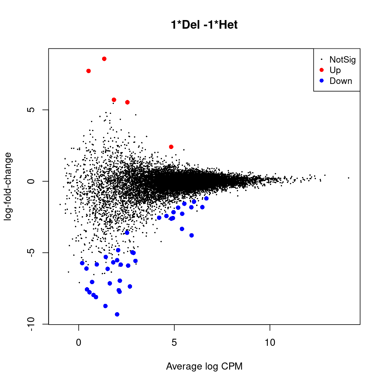
Show code

y_dgeglm <- glmFit(y, y_design)
y_contrast <- makeContrasts(Del - Het, levels = y_design)
y_dgelrt <- glmLRT(y_dgeglm, contrast = y_contrast)
y_dt <- decideTests(y_dgelrt)

summary(y_dt) %>%
  knitr::kable(caption = "Number of DEGs (FDR < 0.05)")

Table 1: Number of DEGs (FDR < 0.05)

	1Del -1Het
Down	78
NotSig	11362
Up	10

Show code

par(mfrow = c(1, 1))
plotMD(y_dgelrt)

Figure 6: MD plot highlighting DEGs (red).

An interactive Glimma MD plot of the differential expression results is available from output/DEGs/reads/glimma-plots/aggregated_tech_reps.md-plot.html.

Show code

glMDPlot(
  x = y_dgelrt,
  counts = y,
  anno = y$genes,
  display.columns = c("ENSEMBL.SYMBOL"),
  groups = y$samples$group,
  samples = colnames(y),
  status = y_dt,
  transform = TRUE,
  sample.cols = y$samples$smchd1_genotype_updated_colours,
  path = outdir,
  html = "aggregated_tech_reps.md-plot",
  launch = FALSE)

Show code

y_tt <- topTags(y_dgelrt, p.value = 0.05, n = Inf)
if (nrow(y_tt)) {
  y_tt$table[, c("logFC", "logCPM", "LR", "PValue", "FDR")] %>%
    DT::datatable(caption = "DEGs (FDR < 0.05)") %>%
    DT::formatSignif(
      c("logFC", "logCPM", "LR", "PValue", "FDR"),
      digits = 3)
}

CSV file of results available from output/DEGs/reads/.

Show code

gzout <- gzfile(
  description = file.path(outdir, "aggregated_tech_reps.DEGs.csv.gz"),
  open = "wb")
write.csv(
  topTags(y_dgelrt, n = Inf),
  gzout,
  # NOTE: quote = TRUE needed because some fields contain commas.
  quote = TRUE,
  row.names = FALSE)
close(gzout)

Figure 7 is a heatmap showing the expression of the DEGs.

Show code

pheatmap(
  cpm(y, log = TRUE)[rownames(y_tt), ],
  cluster_rows = TRUE,
  cluster_cols = FALSE,
  color = hcl.colors(101, "Blue-Red 3"),
  breaks = seq(-3, 3, length.out = 101),
  scale = "row",
  annotation_col = data.frame(
    genotype = y$samples$smchd1_genotype_updated,
    sex = y$samples$sex,
    row.names = colnames(y)),
  annotation_colors = list(
    genotype = smchd1_genotype_updated_colours,
    sex = sex_colours),
  main = "Male and female samples",
  fontsize = 9)

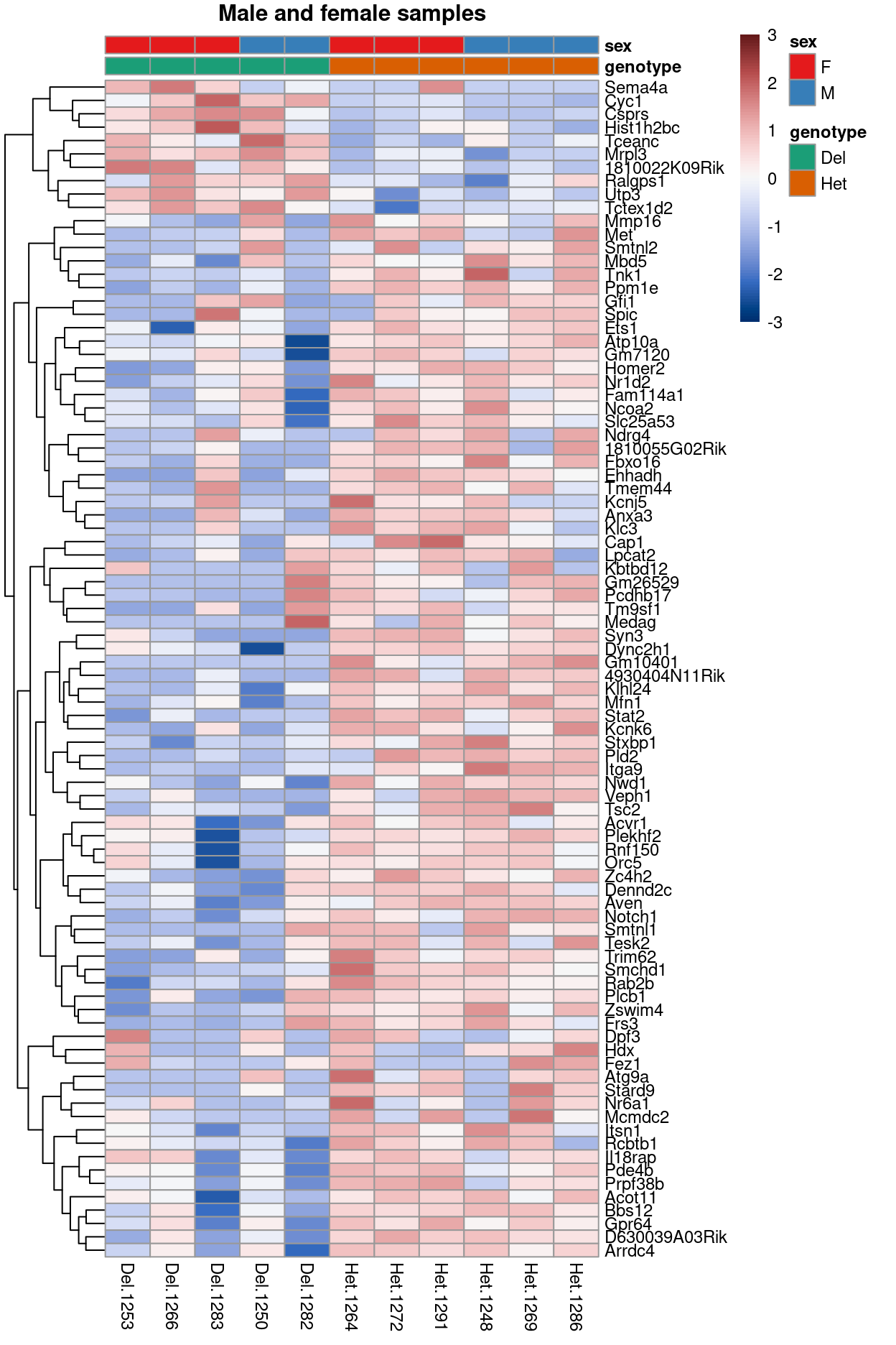
Figure 7: Heatmap of upper-quartile-normalized logCPM values for the DEGs.

Gene set tests

Gene set testing is commonly used to interpret the differential expression results in a biological context. Here we apply various gene set tests to the DEG lists.

goana

We use the goana() function from the limma R/Bioconductor package to test for over-representation of gene ontology (GO) terms in each DEG list.

Show code

list_of_go <- lapply(colnames(y_contrast), function(j) {
  dgelrt <- glmLRT(y_dgeglm, contrast = y_contrast[, j])
  
  go <- goana(
    de = dgelrt,
    geneid = sapply(strsplit(dgelrt$genes$NCBI.ENTREZID, "; "), "[[", 1),
    species = "Mm")
  gzout <- gzfile(
    description = file.path(outdir, "aggregated_tech_reps.goana.csv.gz"),
    open = "wb")
  write.csv(
    topGO(go, number = Inf),
    gzout,
    row.names = TRUE)
  close(gzout)
  go
})
names(list_of_go) <- colnames(y_contrast)

CSV files of the results are available from output/DEGs/reads/.

An example of the results are shown below.

Show code

topGO(list_of_go[[1]]) %>%
  knitr::kable(
    caption = '`goana()` produces a table with a row for each GO term and the following columns: **Term** (GO term); **Ont** (ontology that the GO term belongs to. Possible values are "BP", "CC" and "MF"); **N** (number of genes in the GO term); **Up** (number of up-regulated differentially expressed genes); **Down** (number of down-regulated differentially expressed genes); **P.Up** (p-value for over-representation of GO term in up-regulated genes); **P.Down** (p-value for over-representation of GO term in down-regulated genes)')

Table 2: goana() produces a table with a row for each GO term and the following columns: Term (GO term); Ont (ontology that the GO term belongs to. Possible values are “BP,” “CC” and “MF”); N (number of genes in the GO term); Up (number of up-regulated differentially expressed genes); Down (number of down-regulated differentially expressed genes); P.Up (p-value for over-representation of GO term in up-regulated genes); P.Down (p-value for over-representation of GO term in down-regulated genes)

	Term	Ont	N	Up	Down	P.Up	P.Down
GO:0007610	behavior	BP	330	0	10	1.0000000	0.0000743
GO:0005886	plasma membrane	CC	2383	2	31	0.6545710	0.0000942
GO:0008277	regulation of G protein-coupled receptor signaling pathway	BP	73	0	5	1.0000000	0.0001331
GO:0071944	cell periphery	CC	2469	2	31	0.6758572	0.0001873
GO:0006928	movement of cell or subcellular component	BP	1156	2	19	0.2716901	0.0002006
GO:0060956	endocardial cell differentiation	BP	4	0	2	1.0000000	0.0002710
GO:0060046	regulation of acrosome reaction	BP	4	0	2	1.0000000	0.0002710
GO:0003348	cardiac endothelial cell differentiation	BP	5	0	2	1.0000000	0.0004497
GO:0061343	cell adhesion involved in heart morphogenesis	BP	5	0	2	1.0000000	0.0004497
GO:0045597	positive regulation of cell differentiation	BP	670	0	13	1.0000000	0.0005275
GO:0072148	epithelial cell fate commitment	BP	6	0	2	1.0000000	0.0006717
GO:0062043	positive regulation of cardiac epithelial to mesenchymal transition	BP	6	0	2	1.0000000	0.0006717
GO:0062042	regulation of cardiac epithelial to mesenchymal transition	BP	6	0	2	1.0000000	0.0006717
GO:0010717	regulation of epithelial to mesenchymal transition	BP	59	0	4	1.0000000	0.0006757
GO:0051239	regulation of multicellular organismal process	BP	1844	1	24	0.8308213	0.0008459
GO:0045153	electron transporter, transferring electrons within CoQH2-cytochrome c reductase complex activity	MF	1	1	0	0.0008825	1.0000000
GO:0005887	integral component of plasma membrane	CC	452	1	10	0.3344946	0.0009219
GO:0060973	cell migration involved in heart development	BP	7	0	2	1.0000000	0.0009362
GO:0003198	epithelial to mesenchymal transition involved in endocardial cushion formation	BP	7	0	2	1.0000000	0.0009362
GO:0005523	tropomyosin binding	MF	7	0	2	1.0000000	0.0009362

kegga

We use the kegga() function from the limma R/Bioconductor package to test for over-representation of KEGG pathways in each DEG list.

Show code

list_of_kegg <- lapply(colnames(y_contrast), function(j) {
  dgelrt <- glmLRT(y_dgeglm, contrast = y_contrast[, j])
  
  kegg <- kegga(
    de = dgelrt,
    geneid = sapply(strsplit(dgelrt$genes$NCBI.ENTREZID, "; "), "[[", 1),
    species = "Mm")
  gzout <- gzfile(
    description = file.path(outdir, "aggregated_tech_reps.kegga.csv.gz"),
    open = "wb")
  write.csv(
    topKEGG(kegg, number = Inf),
    gzout,
    row.names = TRUE)
  close(gzout)
  kegg
})
names(list_of_kegg) <- colnames(y_contrast)

CSV files of the results are available from output/DEGs/reads/.

An example of the results are shown below.

Show code

topKEGG(list_of_kegg[[1]]) %>%
  knitr::kable(
    caption = '`kegga()` produces a table with a row for each KEGG pathway ID and the following columns: **Pathway** (KEGG pathway); **N** (number of genes in the GO term); **Up** (number of up-regulated differentially expressed genes); **Down** (number of down-regulated differentially expressed genes); **P.Up** (p-value for over-representation of KEGG pathway in up-regulated genes); **P.Down** (p-value for over-representation of KEGG pathway in down-regulated genes)')

Table 3: kegga() produces a table with a row for each KEGG pathway ID and the following columns: Pathway (KEGG pathway); N (number of genes in the GO term); Up (number of up-regulated differentially expressed genes); Down (number of down-regulated differentially expressed genes); P.Up (p-value for over-representation of KEGG pathway in up-regulated genes); P.Down (p-value for over-representation of KEGG pathway in down-regulated genes)

	Pathway	N	Up	Down	P.Up	P.Down
path:mmu04928	Parathyroid hormone synthesis, secretion and action	72	0	4	1.0000000	0.0014987
path:mmu04919	Thyroid hormone signaling pathway	95	0	4	1.0000000	0.0041173
path:mmu04724	Glutamatergic synapse	58	0	3	1.0000000	0.0073758
path:mmu00565	Ether lipid metabolism	24	0	2	1.0000000	0.0117017
path:mmu04915	Estrogen signaling pathway	80	0	3	1.0000000	0.0176377
path:mmu04929	GnRH secretion	37	0	2	1.0000000	0.0266607
path:mmu04072	Phospholipase D signaling pathway	101	0	3	1.0000000	0.0323083
path:mmu05032	Morphine addiction	42	0	2	1.0000000	0.0337172
path:mmu05200	Pathways in cancer	352	0	6	1.0000000	0.0340336
path:mmu04260	Cardiac muscle contraction	47	1	0	0.0407222	1.0000000
path:mmu04726	Serotonergic synapse	52	0	2	1.0000000	0.0497017
path:mmu04713	Circadian entrainment	53	0	2	1.0000000	0.0514257
path:mmu04621	NOD-like receptor signaling pathway	123	0	3	1.0000000	0.0527650
path:mmu04925	Aldosterone synthesis and secretion	55	0	2	1.0000000	0.0549374
path:mmu05206	MicroRNAs in cancer	129	0	3	1.0000000	0.0592099
path:mmu05322	Systemic lupus erythematosus	75	1	0	0.0642668	1.0000000
path:mmu05165	Human papillomavirus infection	221	0	4	1.0000000	0.0657841
path:mmu04014	Ras signaling pathway	136	0	3	1.0000000	0.0671756
path:mmu05211	Renal cell carcinoma	62	0	2	1.0000000	0.0678581
path:mmu00564	Glycerophospholipid metabolism	65	0	2	1.0000000	0.0736747

camera with MSigDB gene sets

We use the camera() function from the limma R/Bioconductor package to test whether a set of genes is highly ranked relative to other genes in terms of differential expression, accounting for inter-gene correlation. Specifically, we test using gene sets from MSigDB, namely:

We download these gene sets from http://bioinf.wehi.edu.au/MSigDB/index.html

• H: hallmark gene sets are coherently expressed signatures derived by aggregating many MSigDB gene sets to represent well-defined biological states or processes.
• C2: curated gene sets from online pathway databases, publications in PubMed, and knowledge of domain experts.

Show code

# NOTE: Using BiocFileCache to avoid re-downloading these gene sets everytime 
#       the report is rendered.
library(BiocFileCache)
bfc <- BiocFileCache()
# NOTE: Creating list of gene sets in this slightly convoluted way so that each 
#       gene set name is prepended by its origin (e.g. H, C2, or C7).
msigdb <- do.call(
  c, 
  list(
    H = readRDS(
      bfcrpath(
        bfc,
        "http://bioinf.wehi.edu.au/MSigDB/v7.1/Mm.h.all.v7.1.entrez.rds")),
    C2 = readRDS(
      bfcrpath(
        bfc, 
        "http://bioinf.wehi.edu.au/MSigDB/v7.1/Mm.c2.all.v7.1.entrez.rds"))))

y_idx <- ids2indices(
  msigdb, 
  id = sapply(strsplit(y$genes$NCBI.ENTREZID, "; "), "[[", 1))
list_of_camera <- lapply(colnames(y_contrast), function(j) {
  cam <- camera(
    y = y, 
    index = y_idx,
    design = y_design, 
    contrast = y_contrast[, j])
  gzout <- gzfile(
    description = file.path(outdir, "aggregated_tech_reps.camera.csv.gz"),
    open = "wb")
  write.csv(
    cam,
    gzout,
    row.names = TRUE)
  close(gzout)
  cam
})
names(list_of_camera) <- colnames(y_contrast)

CSV files of the results are available from output/DEGs/reads.

An example of the results are shown below.

Show code

head(list_of_camera[[1]]) %>%
  knitr::kable(
    caption = '`camera()` produces a table with a row for each gene set (prepended by which MSigDB collection it comes from) and the following columns: **NGenes** (number of genes in set); **Direction** (direction of change); **PValue** (two-tailed p-value); **FDR** (Benjamini and Hochberg FDR adjusted p-value).')

Table 4: camera() produces a table with a row for each gene set (prepended by which MSigDB collection it comes from) and the following columns: NGenes (number of genes in set); Direction (direction of change); PValue (two-tailed p-value); FDR (Benjamini and Hochberg FDR adjusted p-value).

	NGenes	Direction	PValue	FDR
C2.KEGG_RIBOSOME	102	Up	0	6.0e-07
C2.REACTOME_EUKARYOTIC_TRANSLATION_ELONGATION	107	Up	0	2.3e-06
C2.REACTOME_SRP_DEPENDENT_COTRANSLATIONAL_PROTEIN_TARGETING_TO_MEMBRANE	130	Up	0	4.4e-06
C2.REACTOME_RESPIRATORY_ELECTRON_TRANSPORT_ATP_SYNTHESIS_BY_CHEMIOSMOTIC_COUPLING_AND_HEAT_PRODUCTION_BY_UNCOUPLING_PROTEINS	120	Up	0	4.4e-06
C2.REACTOME_RESPONSE_OF_EIF2AK4_GCN2_TO_AMINO_ACID_DEFICIENCY	115	Up	0	4.4e-06
C2.REACTOME_EUKARYOTIC_TRANSLATION_INITIATION	139	Up	0	4.4e-06

Sarah’s gene lists

Show code

y_X <- y$genes$ENSEMBL.SEQNAME == "X"
y_protocadherin <- grepl("Pcdh", rownames(y))
y_pw <- rownames(y) %in% c("Ndn", "Mkrn3", "Peg12")
y_male <- male_het_vs_del[
  male_het_vs_del$FDR < 0.05,
  c("ENSEMBL.SYMBOL", "logFC")]
y_female <- male_het_vs_del[
  female_het_vs_del$FDR < 0.05,
  c("ENSEMBL.SYMBOL", "logFC")]
y_sun <- sun_2014[, c("geneSymbol", "log2FC")]
y_chambers <- chambers_2007[, c("Gene Symbol", "Fold Difference")]
y_chambers$logFC <- log2(y_chambers$`Fold Difference`)
y_chambers$`Fold Difference` <- NULL
y_chambers <- y_chambers[!is.na(y_chambers$`Gene Symbol`), ]
y_chambers <- y_chambers[!duplicated(y_chambers$`Gene Symbol`), ]
y_gazit <- gazit_2013[, c("Symbol"), drop = FALSE]
y_gazit$Symbol <- paste(
  substring(y_gazit$Symbol, 1, 1), 
  tolower(substring(y_gazit$Symbol, 2)),
  sep = "")
y_gazit$logFC <- 1
y_chambers_gazit <- data.frame(
  Symbol = c(y_chambers$`Gene Symbol`, y_gazit$Symbol),
  logFC = c(y_chambers$logFC, y_gazit$logFC))
y_chambers_gazit <- y_chambers_gazit[!duplicated(y_chambers_gazit$Symbol), ]
y_venezia_proliferation <- rownames(y) %in% venezia_proliferation$Gene.Symbol
y_venezia_quiescence <- rownames(y) %in% venezia_quiescence$Gene.Symbol

y_index <- list(
  `X-linked` = y_X,
  Protocadherin = y_protocadherin,
  `Prader-Willi` = y_pw,
  `Male: Het vs. Del` = y_male,
  `Female: Het vs. Del` = y_female,
  `Sun (2014)` = y_sun,
  `Chambers (2007)` = y_chambers,
  `Gazit (2013)` = y_gazit,
  `Chambers (2007) & Gazit (2013)` = y_chambers_gazit,
  `Proliferation Group Venezia (2004)` = y_venezia_proliferation,
  `Quiescence Group Venezia (2004)` = y_venezia_quiescence)

Sarah requested testing a number of gene sets (see Gene sets).

We use the fry() function from the edgeR R/Bioconductor package to perform a self-contained gene set test against the null hypothesis that none of the genes in the set are differentially expressed.

Show code

fry(
  y,
  index = y_index,
  design = y_design,
  contrast = y_contrast, 
  sort = "none") %>%
    knitr::kable(
      caption = "Results of applying `fry()` to the RNA-seq differential expression results using the supplied gene sets. A significant 'Up' P-value means that the differential expression results found in the RNA-seq data are positively correlated with the expression signature from the corresponding gene set. Conversely, a significant 'Down' P-value means that the differential expression log-fold-changes are negatively correlated with the expression signature from the corresponding gene set. A significant 'Mixed' P-value means that the genes in the set tend to be differentially expressed without regard for direction.")

Table 5: Results of applying fry() to the RNA-seq differential expression results using the supplied gene sets. A significant ‘Up’ P-value means that the differential expression results found in the RNA-seq data are positively correlated with the expression signature from the corresponding gene set. Conversely, a significant ‘Down’ P-value means that the differential expression log-fold-changes are negatively correlated with the expression signature from the corresponding gene set. A significant ‘Mixed’ P-value means that the genes in the set tend to be differentially expressed without regard for direction.

	NGenes	Direction	PValue	FDR	PValue.Mixed	FDR.Mixed
X-linked	388	Down	0.4732142	0.4732142	0.0000240	0.0002641
Protocadherin	4	Down	0.1818142	0.2499945	0.0359534	0.0395488
Prader-Willi	3	Up	0.2856524	0.3491307	0.4549877	0.4549877
Male: Het vs. Del	7	Up	0.0159925	0.0433171	0.0000583	0.0003203
Female: Het vs. Del	17	Up	0.1731703	0.2499945	0.0001075	0.0003203
Sun (2014)	1997	Down	0.3728438	0.4101281	0.0004929	0.0007745
Chambers (2007)	208	Down	0.0036999	0.0289609	0.0001395	0.0003203
Gazit (2013)	249	Down	0.0430404	0.0789075	0.0094767	0.0115826
Chambers (2007) & Gazit (2013)	404	Down	0.0066715	0.0289609	0.0001456	0.0003203
Proliferation Group Venezia (2004)	365	Up	0.0078984	0.0289609	0.0009692	0.0013326
Quiescence Group Venezia (2004)	382	Down	0.0196896	0.0433171	0.0003511	0.0006437

Show code

par(mfrow = c(length(y_index), 2))
for (n in names(y_index)) {
  if (is.data.frame(y_index[[n]])) {
    y_status <- rep(0, nrow(y_dgelrt))
    y_status[rownames(y) %in% y_index[[n]][, 1]] <-
      sign(y_index[[n]][y_index[[n]][, 1] %in% rownames(y), 2])
    plotMD(
      y_dgelrt,
      status = y_status,
      hl.col = c("red", "blue"),
      legend = "bottomright",
      main = n)
    abline(h = 0, col = "darkgrey")
  } else {
    y_status <- rep("Other", nrow(y_dgelrt))
    y_status[y_index[[n]]] <- n
    plotMD(
      y_dgelrt,
      status = y_status,
      values = n,
      hl.col = "red",
      legend = "bottomright",
      main = n)
    abline(h = 0, col = "darkgrey")
  }
  
  if (is.data.frame(y_index[[n]])) {
    barcodeplot(
      y_dgelrt$table$logFC,
      rownames(y) %in% y_index[[n]][, 1],
      gene.weights = y_index[[n]][
        y_index[[n]][, 1] %in% rownames(y), 2])
  } else {
    barcodeplot(
      y_dgelrt$table$logFC,
      y_index[[n]])
  }
}

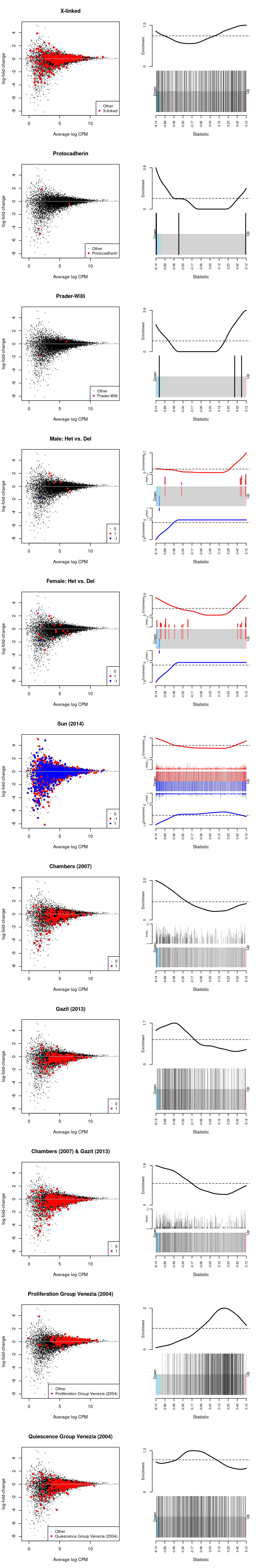
Figure 8: MD-plot and barcode plot of DEGs in supplied gene sets. Directional gene sets have (1) MD plot points coloured according to the statistical significance of the gene in the gene set (2) barcode plot ‘weights’ given by the logFC of the gene in the gene set. For the barcode plot, genes are represented by bars and are ranked from left to right by increasing log-fold change. This forms the barcode-like pattern. The line (or worm) above the barcode shows the relative local enrichment of the vertical bars in each part of the plot. The dotted horizontal line indicates neutral enrichment; the worm above the dotted line shows enrichment while the worm below the dotted line shows depletion.

Male-only: analysis of aggregated technical replicates

Show code

ym_differences <- makeGroups(ym$samples$smchd1_genotype_updated)
ym_ruv <- RUVs(
    x = betweenLaneNormalization(ym$counts, "upper"),
    cIdx = rownames(ym),
    k = 1,
    scIdx = ym_differences)

ym_design <- model.matrix(
  ~0 + smchd1_genotype_updated + ym_ruv$W,
  ym$samples)
colnames(ym_design) <- sub(
  "ruv\\$|smchd1_genotype_updated",
  "",
  colnames(ym_design))

MDS

Show code

ym_mds <- plotMDS(cpm(ym_ruv$normalizedCounts, log = TRUE), plot = FALSE)

ym_df <- cbind(data.frame(x = ym_mds$x, y = ym_mds$y), ym$samples)
rownames(ym_df) <- colnames(ym)

p1 <- ggplot(
  aes(x = x, y = y, colour = smchd1_genotype_updated, label = rownames(ym_df)),
  data = ym_df) +
  geom_point() +
  geom_text_repel(size = 2) +
  theme_cowplot(font_size = 8) +
  xlab("Leading logFC dim 1") +
  ylab("Leading logFC dim 2") +
  scale_colour_manual(values = smchd1_genotype_updated_colours)
p2 <- ggplot(
  aes(x = x, y = y, colour = sex, label = rownames(ym_df)),
  data = ym_df) +
  geom_point() +
  geom_text_repel(size = 2) +
  theme_cowplot(font_size = 8) +
  xlab("Leading logFC dim 1") +
  ylab("Leading logFC dim 2") +
  scale_colour_manual(values = sex_colours)
p3 <- ggplot(
  aes(x = x, y = y, colour = mouse_number, label = rownames(ym_df)),
  data = ym_df) +
  geom_point() +
  geom_text_repel(size = 2) +
  theme_cowplot(font_size = 8) +
  xlab("Leading logFC dim 1") +
  ylab("Leading logFC dim 2") +
  scale_colour_manual(values = mouse_number_colours)
p4 <- ggplot(
  aes(x = x, y = y, colour = log10(lib.size), label = rownames(ym_df)),
  data = ym_df) +
  geom_point() +
  geom_text_repel(size = 2) +
  theme_cowplot(font_size = 8) +
  scale_colour_viridis_c() +
  xlab("Leading logFC dim 1") +
  ylab("Leading logFC dim 2")

p1 + p2 + p3 + p4 + plot_layout(ncol = 2)

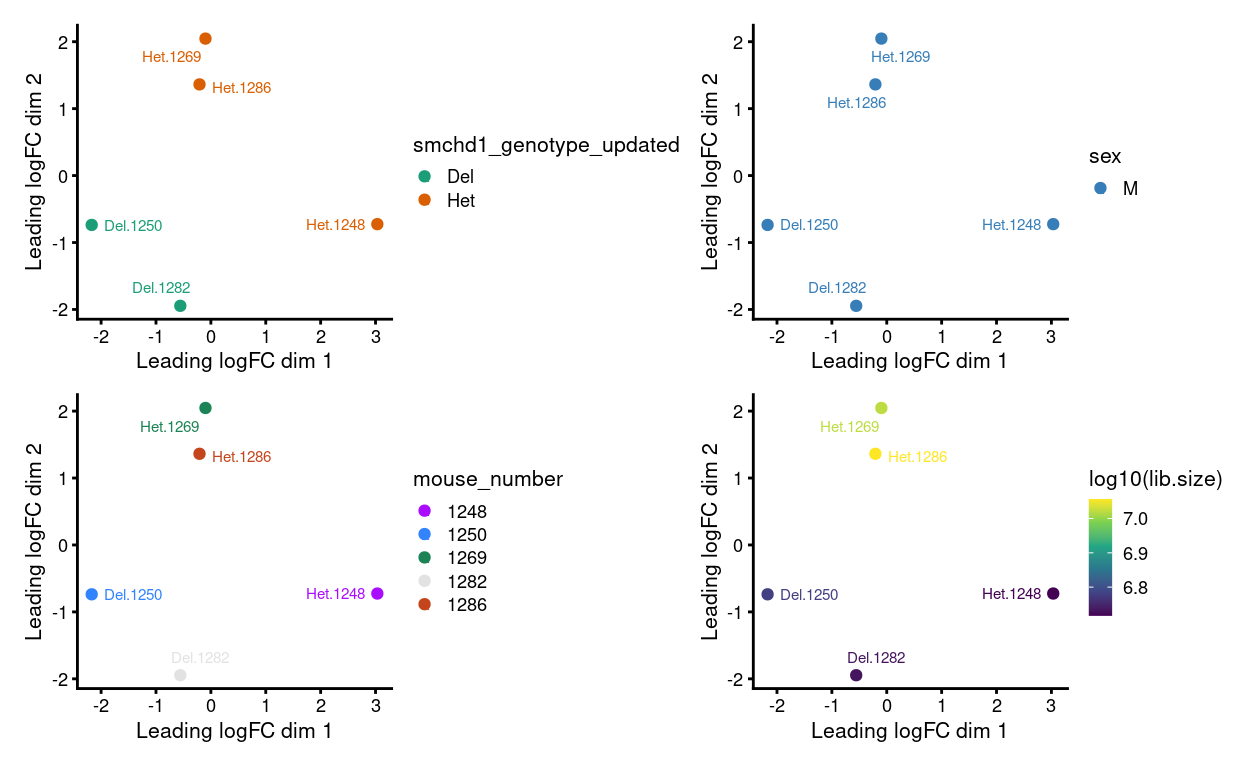
Figure 9: MDS plots of aggregated technical replicates following RUV coloured by various experimental factors.

DE analysis

Fit a model using edgeR with a term for smchd1_genotype_updated.

Show code

ym <- estimateDisp(ym, ym_design)
par(mfrow = c(1, 1))
plotBCV(ym)

Show code

ym_dgeglm <- glmFit(ym, ym_design)
ym_contrast <- makeContrasts(Del - Het, levels = ym_design)
ym_dgelrt <- glmLRT(ym_dgeglm, contrast = ym_contrast)
ym_dt <- decideTests(ym_dgelrt)

summary(ym_dt) %>%
  knitr::kable(caption = "Number of DEGs (FDR < 0.05)")

Table 6: Number of DEGs (FDR < 0.05)

	1Del -1Het
Down	44
NotSig	11543
Up	12

Show code

par(mfrow = c(1, 1))
plotMD(ym_dgelrt)

Figure 10: MD plot highlighting DEGs (red).

An interactive Glimma MD plot of the differential expression results is available from output/DEGs/reads/glimma-plots/aggregated_tech_reps.males.md-plot.html.

Show code

ym_tt <- topTags(ym_dgelrt, n = Inf, sort.by = "none")
glMDPlot(
  x = ym_dgelrt,
  counts = ym,
  anno = ym$genes,
  display.columns = c("ENSEMBL.SYMBOL"),
  groups = ym$samples$group,
  samples = colnames(ym),
  status = ym_dt,
  transform = TRUE,
  sample.cols = ym$samples$smchd1_genotype_updated_colours,
  path = outdir,
  html = "aggregated_tech_reps.males.md-plot",
  launch = FALSE)

Show code

ym_tt <- topTags(ym_dgelrt, p.value = 0.05, n = Inf)
if (nrow(ym_tt)) {
  ym_tt$table[, c("logFC", "logCPM", "LR", "PValue", "FDR")] %>%
    DT::datatable(caption = "DEGs (FDR < 0.05)") %>%
    DT::formatSignif(
      c("logFC", "logCPM", "LR", "PValue", "FDR"),
      digits = 3)
}

CSV file of results available from output/DEGs/reads/aggregated_tech_reps.males.DEGs.csv.gz.

Show code

gzout <- gzfile(
  description = file.path(outdir, "aggregated_tech_reps.males.DEGs.csv.gz"),
  open = "wb")
write.csv(
  topTags(ym_dgelrt, n = Inf),
  gzout,
  # NOTE: quote = TRUE needed because some fields contain commas.
  quote = TRUE,
  row.names = FALSE)
close(gzout)

Figure 11 is a heatmap showing the expression of the DEGs.

Show code

pheatmap(
  cpm(ym, log = TRUE)[rownames(ym_tt), ],
  cluster_rows = TRUE,
  cluster_cols = FALSE,
  color = hcl.colors(101, "Blue-Red 3"),
  breaks = seq(-3, 3, length.out = 101),
  scale = "row",
  annotation_col = data.frame(
    genotype = ym$samples$smchd1_genotype_updated,
    sex = ym$samples$sex,
    row.names = colnames(ym)),
  annotation_colors = list(
    genotype = smchd1_genotype_updated_colours,
    sex = sex_colours),
  main = "Male samples",
  fontsize = 9)

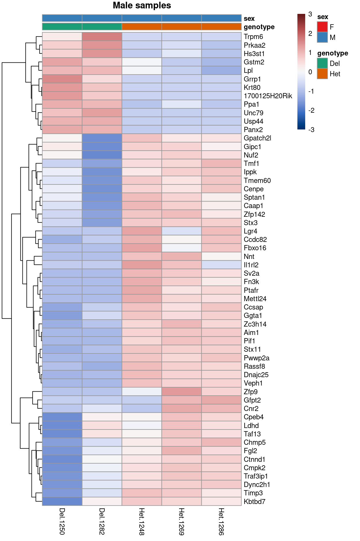
Figure 11: Heatmap of upper-quartile-normalzied logCPM values for the DEGs.

Gene set tests

Gene set testing is commonly used to interpret the differential expression results in a biological context. Here we apply various gene set tests to the DEG lists.

goana

We use the goana() function from the limma R/Bioconductor package to test for over-representation of gene ontology (GO) terms in each DEG list.

Show code

list_of_go <- lapply(colnames(ym_contrast), function(j) {
  dgelrt <- glmLRT(ym_dgeglm, contrast = ym_contrast[, j])
  
  go <- goana(
    de = dgelrt,
    geneid = sapply(strsplit(dgelrt$genes$NCBI.ENTREZID, "; "), "[[", 1),
    species = "Mm")
  gzout <- gzfile(
    description = file.path(outdir, "aggregated_tech_reps.males.goana.csv.gz"),
    open = "wb")
  write.csv(
    topGO(go, number = Inf),
    gzout,
    row.names = TRUE)
  close(gzout)
  go
})
names(list_of_go) <- colnames(ym_contrast)

CSV files of the results are available from output/DEGs/reads/.

An example of the results are shown below.

Show code

topGO(list_of_go[[1]]) %>%
  knitr::kable(
    caption = '`goana()` produces a table with a row for each GO term and the following columns: **Term** (GO term); **Ont** (ontology that the GO term belongs to. Possible values are "BP", "CC" and "MF"); **N** (number of genes in the GO term); **Up** (number of up-regulated differentially expressed genes); **Down** (number of down-regulated differentially expressed genes); **P.Up** (p-value for over-representation of GO term in up-regulated genes); **P.Down** (p-value for over-representation of GO term in down-regulated genes)')

Table 7: goana() produces a table with a row for each GO term and the following columns: Term (GO term); Ont (ontology that the GO term belongs to. Possible values are “BP,” “CC” and “MF”); N (number of genes in the GO term); Up (number of up-regulated differentially expressed genes); Down (number of down-regulated differentially expressed genes); P.Up (p-value for over-representation of GO term in up-regulated genes); P.Down (p-value for over-representation of GO term in down-regulated genes)

	Term	Ont	N	Up	Down	P.Up	P.Down
GO:0048786	presynaptic active zone	CC	48	0	4	1.0000000	0.0000323
GO:0006633	fatty acid biosynthetic process	BP	92	3	0	0.0001039	1.0000000
GO:0016079	synaptic vesicle exocytosis	BP	70	0	4	1.0000000	0.0001431
GO:0099568	cytoplasmic region	CC	134	0	5	1.0000000	0.0001514
GO:0072330	monocarboxylic acid biosynthetic process	BP	113	3	0	0.0001914	1.0000000
GO:0071398	cellular response to fatty acid	BP	21	2	0	0.0002080	1.0000000
GO:0045055	regulated exocytosis	BP	147	0	5	1.0000000	0.0002334
GO:0043207	response to external biotic stimulus	BP	715	1	10	0.5378743	0.0002948
GO:0051707	response to other organism	BP	715	1	10	0.5378743	0.0002948
GO:0009607	response to biotic stimulus	BP	739	1	10	0.5500911	0.0003843
GO:0007269	neurotransmitter secretion	BP	94	0	4	1.0000000	0.0004451
GO:0099643	signal release from synapse	BP	94	0	4	1.0000000	0.0004451
GO:0070542	response to fatty acid	BP	31	2	0	0.0004578	1.0000000
GO:0007080	mitotic metaphase plate congression	BP	40	0	3	1.0000000	0.0004699
GO:0032838	plasma membrane bounded cell projection cytoplasm	CC	102	0	4	1.0000000	0.0006066
GO:0007052	mitotic spindle organization	BP	103	0	4	1.0000000	0.0006294
GO:0043312	neutrophil degranulation	BP	10	0	2	1.0000000	0.0006334
GO:0030425	dendrite	CC	395	1	7	0.3431457	0.0006892
GO:0097447	dendritic tree	CC	396	1	7	0.3438566	0.0006996
GO:0046394	carboxylic acid biosynthetic process	BP	184	3	0	0.0008007	1.0000000

kegga

We use the kegga() function from the limma R/Bioconductor package to test for over-representation of KEGG pathways in each DEG list.

Show code

list_of_kegg <- lapply(colnames(ym_contrast), function(j) {
  dgelrt <- glmLRT(ym_dgeglm, contrast = ym_contrast[, j])
  
  kegg <- kegga(
    de = dgelrt,
    geneid = sapply(strsplit(dgelrt$genes$NCBI.ENTREZID, "; "), "[[", 1),
    species = "Mm")
  gzout <- gzfile(
    description = file.path(outdir, "aggregated_tech_reps.males.kegga.csv.gz"),
    open = "wb")
  write.csv(
    topKEGG(kegg, number = Inf),
    gzout,
    row.names = TRUE)
  close(gzout)
  kegg
})
names(list_of_kegg) <- colnames(ym_contrast)

CSV files of the results are available from output/DEGs/reads/.

An example of the results are shown below.

Show code

topKEGG(list_of_kegg[[1]]) %>%
  knitr::kable(
    caption = '`kegga()` produces a table with a row for each KEGG pathway ID and the following columns: **Pathway** (KEGG pathway); **N** (number of genes in the GO term); **Up** (number of up-regulated differentially expressed genes); **Down** (number of down-regulated differentially expressed genes); **P.Up** (p-value for over-representation of KEGG pathway in up-regulated genes); **P.Down** (p-value for over-representation of KEGG pathway in down-regulated genes)')

Table 8: kegga() produces a table with a row for each KEGG pathway ID and the following columns: Pathway (KEGG pathway); N (number of genes in the GO term); Up (number of up-regulated differentially expressed genes); Down (number of down-regulated differentially expressed genes); P.Up (p-value for over-representation of KEGG pathway in up-regulated genes); P.Down (p-value for over-representation of KEGG pathway in down-regulated genes)

	Pathway	N	Up	Down	P.Up	P.Down
path:mmu05418	Fluid shear stress and atherosclerosis	106	2	0	0.0052450	1.0000000
path:mmu04130	SNARE interactions in vesicular transport	31	0	2	1.0000000	0.0062180
path:mmu00534	Glycosaminoglycan biosynthesis - heparan sulfate / heparin	15	1	0	0.0155706	1.0000000
path:mmu04080	Neuroactive ligand-receptor interaction	53	0	2	1.0000000	0.0174721
path:mmu00982	Drug metabolism - cytochrome P450	22	1	0	0.0227606	1.0000000
path:mmu05204	Chemical carcinogenesis - DNA adducts	23	1	0	0.0237838	1.0000000
path:mmu00980	Metabolism of xenobiotics by cytochrome P450	25	1	0	0.0258272	1.0000000
path:mmu04979	Cholesterol metabolism	28	1	0	0.0288851	1.0000000
path:mmu04710	Circadian rhythm	28	1	0	0.0288851	1.0000000
path:mmu04978	Mineral absorption	28	1	0	0.0288851	1.0000000
path:mmu00561	Glycerolipid metabolism	40	1	0	0.0410286	1.0000000
path:mmu03320	PPAR signaling pathway	41	1	0	0.0420342	1.0000000
path:mmu05410	Hypertrophic cardiomyopathy	44	1	0	0.0450454	1.0000000
path:mmu00601	Glycosphingolipid biosynthesis - lacto and neolacto series	12	0	1	1.0000000	0.0450454
path:mmu00983	Drug metabolism - other enzymes	46	1	0	0.0470480	1.0000000
path:mmu04213	Longevity regulating pathway - multiple species	48	1	0	0.0490468	1.0000000
path:mmu04920	Adipocytokine signaling pathway	49	1	0	0.0500447	1.0000000
path:mmu00480	Glutathione metabolism	50	1	0	0.0510417	1.0000000
path:mmu01524	Platinum drug resistance	65	1	0	0.0658817	1.0000000
path:mmu04211	Longevity regulating pathway	71	1	0	0.0717580	1.0000000

camera with MSigDB gene sets

We use the camera() function from the limma R/Bioconductor package to test whether a set of genes is highly ranked relative to other genes in terms of differential expression, accounting for inter-gene correlation. Specifically, we test using gene sets from MSigDB, namely:

We download these gene sets from http://bioinf.wehi.edu.au/MSigDB/index.html

• H: hallmark gene sets are coherently expressed signatures derived by aggregating many MSigDB gene sets to represent well-defined biological states or processes.
• C2: curated gene sets from online pathway databases, publications in PubMed, and knowledge of domain experts.

Show code

ym_idx <- ids2indices(
  msigdb, 
  id = sapply(strsplit(ym$genes$NCBI.ENTREZID, "; "), "[[", 1))
list_of_camera <- lapply(colnames(ym_contrast), function(j) {
  cam <- camera(
    y = ym, 
    index = ym_idx,
    design = ym_design, 
    contrast = ym_contrast[, j])
  gzout <- gzfile(
    description = file.path(outdir, "aggregated_tech_reps.males.camera.csv.gz"),
    open = "wb")
  write.csv(
    cam,
    gzout,
    row.names = TRUE)
  close(gzout)
  cam
})
names(list_of_camera) <- colnames(ym_contrast)

CSV files of the results are available from output/DEGs/reads.

An example of the results are shown below.

Show code

head(list_of_camera[[1]]) %>%
  knitr::kable(
    caption = '`camera()` produces a table with a row for each gene set (prepended by which MSigDB collection it comes from) and the following columns: **NGenes** (number of genes in set); **Direction** (direction of change); **PValue** (two-tailed p-value); **FDR** (Benjamini and Hochberg FDR adjusted p-value).')

Table 9: camera() produces a table with a row for each gene set (prepended by which MSigDB collection it comes from) and the following columns: NGenes (number of genes in set); Direction (direction of change); PValue (two-tailed p-value); FDR (Benjamini and Hochberg FDR adjusted p-value).

	NGenes	Direction	PValue	FDR
H.HALLMARK_MYC_TARGETS_V1	229	Up	0.0000535	0.2203915
C2.JOHANSSON_GLIOMAGENESIS_BY_PDGFB_DN	19	Down	0.0000794	0.2203915
C2.REACTOME_ELECTRIC_TRANSMISSION_ACROSS_GAP_JUNCTIONS	2	Up	0.0001400	0.2592181
C2.RAHMAN_TP53_TARGETS_PHOSPHORYLATED	25	Up	0.0002956	0.3456734
C2.REACTOME_UNWINDING_OF_DNA	12	Up	0.0003112	0.3456734
C2.PID_MYC_ACTIV_PATHWAY	95	Up	0.0003762	0.3482163

Sarah’s gene lists

Show code

ym_X <- ym$genes$ENSEMBL.SEQNAME == "X"
ym_protocadherin <- grepl("Pcdh", rownames(ym))
ym_pw <- rownames(ym) %in% c("Ndn", "Mkrn3", "Peg12")
ym_male <- male_het_vs_del[
  male_het_vs_del$FDR < 0.05,
  c("ENSEMBL.SYMBOL", "logFC")]
ym_female <- male_het_vs_del[
  female_het_vs_del$FDR < 0.05,
  c("ENSEMBL.SYMBOL", "logFC")]
ym_sun <- sun_2014[, c("geneSymbol", "log2FC")]
ym_chambers <- chambers_2007[, c("Gene Symbol", "Fold Difference")]
ym_chambers$logFC <- log2(ym_chambers$`Fold Difference`)
ym_chambers$`Fold Difference` <- NULL
ym_chambers <- ym_chambers[!is.na(ym_chambers$`Gene Symbol`), ]
ym_chambers <- ym_chambers[!duplicated(ym_chambers$`Gene Symbol`), ]
ym_gazit <- gazit_2013[, c("Symbol"), drop = FALSE]
ym_gazit$Symbol <- paste(
  substring(ym_gazit$Symbol, 1, 1), 
  tolower(substring(ym_gazit$Symbol, 2)),
  sep = "")
ym_gazit$logFC <- 1
ym_chambers_gazit <- data.frame(
  Symbol = c(ym_chambers$`Gene Symbol`, ym_gazit$Symbol),
  logFC = c(ym_chambers$logFC, ym_gazit$logFC))
ym_chambers_gazit <- ym_chambers_gazit[!duplicated(ym_chambers_gazit$Symbol), ]
ym_venezia_proliferation <- rownames(ym) %in% venezia_proliferation$Gene.Symbol
ym_venezia_quiescence <- rownames(ym) %in% venezia_quiescence$Gene.Symbol

ym_index <- list(
  `X-linked` = ym_X,
  Protocadherin = ym_protocadherin,
  `Prader-Willi` = ym_pw,
  `Male: Het vs. Del` = ym_male,
  `Female: Het vs. Del` = ym_female,
  `Sun (2014)` = ym_sun,
  `Chambers (2007)` = ym_chambers,
  `Gazit (2013)` = ym_gazit,
  `Chambers (2007) & Gazit (2013)` = ym_chambers_gazit,
  `Proliferation Group Venezia (2004)` = ym_venezia_proliferation,
  `Quiescence Group Venezia (2004)` = ym_venezia_quiescence)

Sarah requested testing a number of gene sets (see Gene sets).

We use the fry() function from the edgeR R/Bioconductor package to perform a self-contained gene set test against the null hypothesis that none of the genes in the set are differentially expressed.

Show code

fry(
  ym, 
  index = ym_index, 
  design = ym_design,
  contrast = ym_contrast,
  sort = "none") %>%
    knitr::kable(
      caption = "Results of applying `fry()` to the RNA-seq differential expression results using the supplied gene sets. A significant 'Up' P-value means that the differential expression results found in the RNA-seq data are positively correlated with the expression signature from the corresponding gene set. Conversely, a significant 'Down' P-value means that the differential expression log-fold-changes are negatively correlated with the expression signature from the corresponding gene set. A significant 'Mixed' P-value means that the genes in the set tend to be differentially expressed without regard for direction.")

Table 10: Results of applying fry() to the RNA-seq differential expression results using the supplied gene sets. A significant ‘Up’ P-value means that the differential expression results found in the RNA-seq data are positively correlated with the expression signature from the corresponding gene set. Conversely, a significant ‘Down’ P-value means that the differential expression log-fold-changes are negatively correlated with the expression signature from the corresponding gene set. A significant ‘Mixed’ P-value means that the genes in the set tend to be differentially expressed without regard for direction.

	NGenes	Direction	PValue	FDR	PValue.Mixed	FDR.Mixed
X-linked	392	Down	0.0346948	0.1056738	0.0085836	0.0157366
Protocadherin	6	Up	0.3718805	0.5843836	0.0278469	0.0437594
Prader-Willi	3	Up	0.5392710	0.6210234	0.0766661	0.0843327
Male: Het vs. Del	8	Up	0.5645667	0.6210234	0.2702930	0.2702930
Female: Het vs. Del	19	Up	0.4705836	0.6210234	0.0074240	0.0157366
Sun (2014)	2023	Up	0.7412489	0.7412489	0.0029447	0.0081364
Chambers (2007)	206	Down	0.0047591	0.0261751	0.0029587	0.0081364
Gazit (2013)	248	Down	0.1999566	0.3665871	0.0007036	0.0077392
Chambers (2007) & Gazit (2013)	402	Down	0.0030405	0.0261751	0.0028950	0.0081364
Proliferation Group Venezia (2004)	364	Up	0.0480335	0.1056738	0.0698494	0.0843327
Quiescence Group Venezia (2004)	383	Down	0.0410618	0.1056738	0.0366139	0.0503441

Show code

par(mfrow = c(length(ym_index), 2))
for (n in names(ym_index)) {
  if (is.data.frame(ym_index[[n]])) {
    ym_status <- rep(0, nrow(ym_dgelrt))
    ym_status[rownames(ym) %in% ym_index[[n]][, 1]] <-
      sign(ym_index[[n]][ym_index[[n]][, 1] %in% rownames(ym), 2])
    plotMD(
      ym_dgelrt,
      status = ym_status,
      hl.col = c("red", "blue"),
      legend = "bottomright",
      main = n)
    abline(h = 0, col = "darkgrey")
  } else {
    ym_status <- rep("Other", nrow(ym_dgelrt))
    ym_status[ym_index[[n]]] <- n
    plotMD(
      ym_dgelrt,
      status = ym_status,
      values = n,
      hl.col = "red",
      legend = "bottomright",
      main = n)
    abline(h = 0, col = "darkgrey")
  }
  
  if (is.data.frame(ym_index[[n]])) {
    barcodeplot(
      ym_dgelrt$table$logFC,
      rownames(ym) %in% ym_index[[n]][, 1],
      gene.weights = ym_index[[n]][
        ym_index[[n]][, 1] %in% rownames(ym), 2])
  } else {
    barcodeplot(
      ym_dgelrt$table$logFC,
      ym_index[[n]])
  }
}

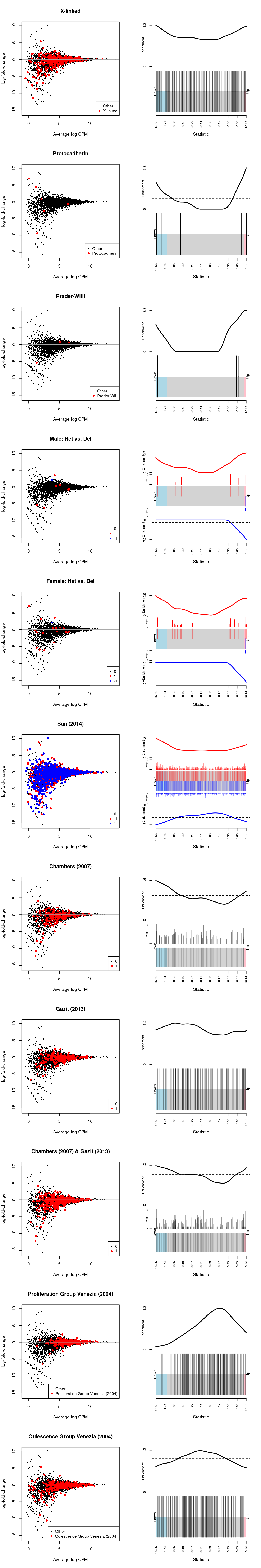
Figure 12: MD-plot and barcode plot of DEGs in supplied gene sets. Directional gene sets have (1) MD plot points coloured according to the statistical significance of the gene in the gene set (2) barcode plot ‘weights’ given by the logFC of the gene in the gene set. For the barcode plot, genes are represented by bars and are ranked from left to right by increasing log-fold change. This forms the barcode-like pattern. The line (or worm) above the barcode shows the relative local enrichment of the vertical bars in each part of the plot. The dotted horizontal line indicates neutral enrichment; the worm above the dotted line shows enrichment while the worm below the dotted line shows depletion.

Female-only: analysis of aggregated technical replicates

Show code

yf_differences <- makeGroups(yf$samples$smchd1_genotype_updated)
yf_ruv <- RUVs(
    x = betweenLaneNormalization(yf$counts, "upper"),
    cIdx = rownames(yf),
    k = 1,
    scIdx = yf_differences)

yf_design <- model.matrix(
  ~0 + smchd1_genotype_updated + yf_ruv$W,
  yf$samples)
colnames(yf_design) <- sub(
  "ruv\\$|smchd1_genotype_updated",
  "",
  colnames(yf_design))

MDS

Show code

yf_mds <- plotMDS(cpm(yf_ruv$normalizedCounts, log = TRUE), plot = FALSE)

yf_df <- cbind(data.frame(x = yf_mds$x, y = yf_mds$y), yf$samples)
rownames(yf_df) <- colnames(yf)

p1 <- ggplot(
  aes(x = x, y = y, colour = smchd1_genotype_updated, label = rownames(yf_df)),
  data = yf_df) +
  geom_point() +
  geom_text_repel(size = 2) +
  theme_cowplot(font_size = 8) +
  xlab("Leading logFC dim 1") +
  ylab("Leading logFC dim 2") +
  scale_colour_manual(values = smchd1_genotype_updated_colours)
p2 <- ggplot(
  aes(x = x, y = y, colour = sex, label = rownames(yf_df)),
  data = yf_df) +
  geom_point() +
  geom_text_repel(size = 2) +
  theme_cowplot(font_size = 8) +
  xlab("Leading logFC dim 1") +
  ylab("Leading logFC dim 2") +
  scale_colour_manual(values = sex_colours)
p3 <- ggplot(
  aes(x = x, y = y, colour = mouse_number, label = rownames(yf_df)),
  data = yf_df) +
  geom_point() +
  geom_text_repel(size = 2) +
  theme_cowplot(font_size = 8) +
  xlab("Leading logFC dim 1") +
  ylab("Leading logFC dim 2") +
  scale_colour_manual(values = mouse_number_colours)
p4 <- ggplot(
  aes(x = x, y = y, colour = log10(lib.size), label = rownames(yf_df)),
  data = yf_df) +
  geom_point() +
  geom_text_repel(size = 2) +
  theme_cowplot(font_size = 8) +
  scale_colour_viridis_c() +
  xlab("Leading logFC dim 1") +
  ylab("Leading logFC dim 2")

p1 + p2 + p3 + p4 + plot_layout(ncol = 2)

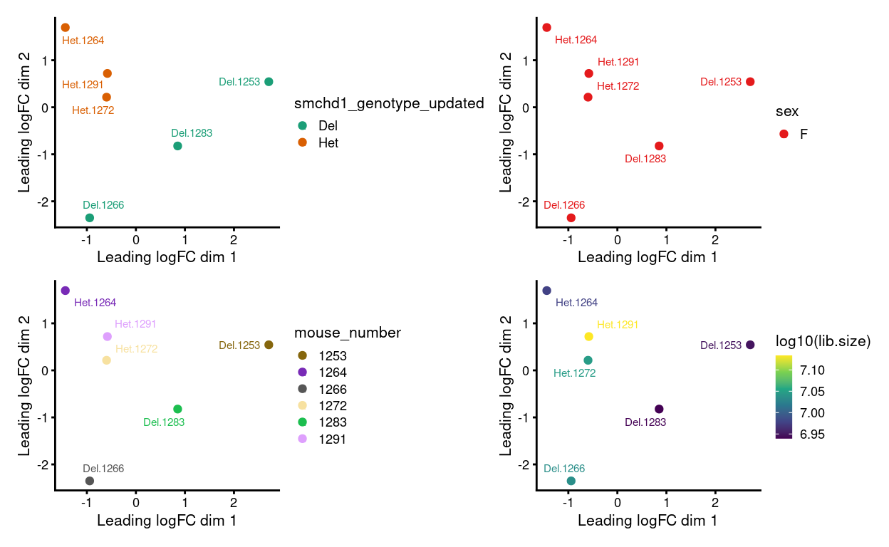
Figure 13: MDS plots of aggregated technical replicates following RUV coloured by various experimental factors.

DE analysis

Fit a model using edgeR with a term for smchd1_genotype_updated.

Show code

yf <- estimateDisp(yf, yf_design)
par(mfrow = c(1, 1))
plotBCV(yf)

Show code

yf_dgeglm <- glmFit(yf, yf_design)
yf_contrast <- makeContrasts(Del - Het, levels = yf_design)
yf_dgelrt <- glmLRT(yf_dgeglm, contrast = yf_contrast)
yf_dt <- decideTests(yf_dgelrt)

summary(yf_dt) %>%
  knitr::kable(caption = "Number of DEGs (FDR < 0.05)")

Table 11: Number of DEGs (FDR < 0.05)

	1Del -1Het
Down	40
NotSig	11468
Up	5

Show code

par(mfrow = c(1, 1))
plotMD(yf_dgelrt)

Figure 14: MD plot highlighting DEGs (red).

An interactive Glimma MD plot of the differential expression results is available from output/DEGs/reads/glimma-plots/aggregated_tech_reps.females.md-plot.html.

Show code

yf_tt <- topTags(yf_dgelrt, n = Inf, sort.by = "none")
glMDPlot(
  x = yf_dgelrt,
  counts = yf,
  anno = yf$genes,
  display.columns = c("ENSEMBL.SYMBOL"),
  groups = yf$samples$group,
  samples = colnames(yf),
  status = yf_dt,
  transform = TRUE,
  sample.cols = yf$samples$smchd1_genotype_updated_colours,
  path = outdir,
  html = "aggregated_tech_reps.females.md-plot",
  launch = FALSE)

Show code

yf_tt <- topTags(yf_dgelrt, p.value = 0.05, n = Inf)
if (nrow(yf_tt)) {
  yf_tt$table[, c("logFC", "logCPM", "LR", "PValue", "FDR")] %>%
    DT::datatable(caption = "DEGs (FDR < 0.05)") %>%
    DT::formatSignif(
      c("logFC", "logCPM", "LR", "PValue", "FDR"),
      digits = 3)
}

CSV file of results available from output/DEGs/reads/aggregated_tech_reps.females.DEGs.csv.gz.

Show code

gzout <- gzfile(
  description = file.path(outdir, "aggregated_tech_reps.females.DEGs.csv.gz"),
  open = "wb")
write.csv(
  topTags(yf_dgelrt, n = Inf),
  gzout,
  # NOTE: quote = TRUE needed because some fields contain commas.
  quote = TRUE,
  row.names = FALSE)
close(gzout)

Show code

heatmapForPaper <- function() {
  pheatmap(
    cpm(yf, log = TRUE)[rownames(yf_tt), ],
    cluster_rows = TRUE,
    cluster_cols = FALSE,
    color = hcl.colors(101, "Blue-Red 3"),
    breaks = seq(-3, 3, length.out = 101),
    scale = "row",
    annotation_col = data.frame(
      genotype = yf$samples$smchd1_genotype_updated,
      sex = yf$samples$sex,
      row.names = colnames(yf)),
    annotation_colors = list(
      genotype = smchd1_genotype_updated_colours,
      sex = sex_colours),
    main = "Female samples",
    fontsize = 9)
}

Figure 15 is a heatmap showing the expression of the DEGs.

A PDF version of this figure is available in output/figures/paper/heatmap.pdf.

Show code

heatmapForPaper()

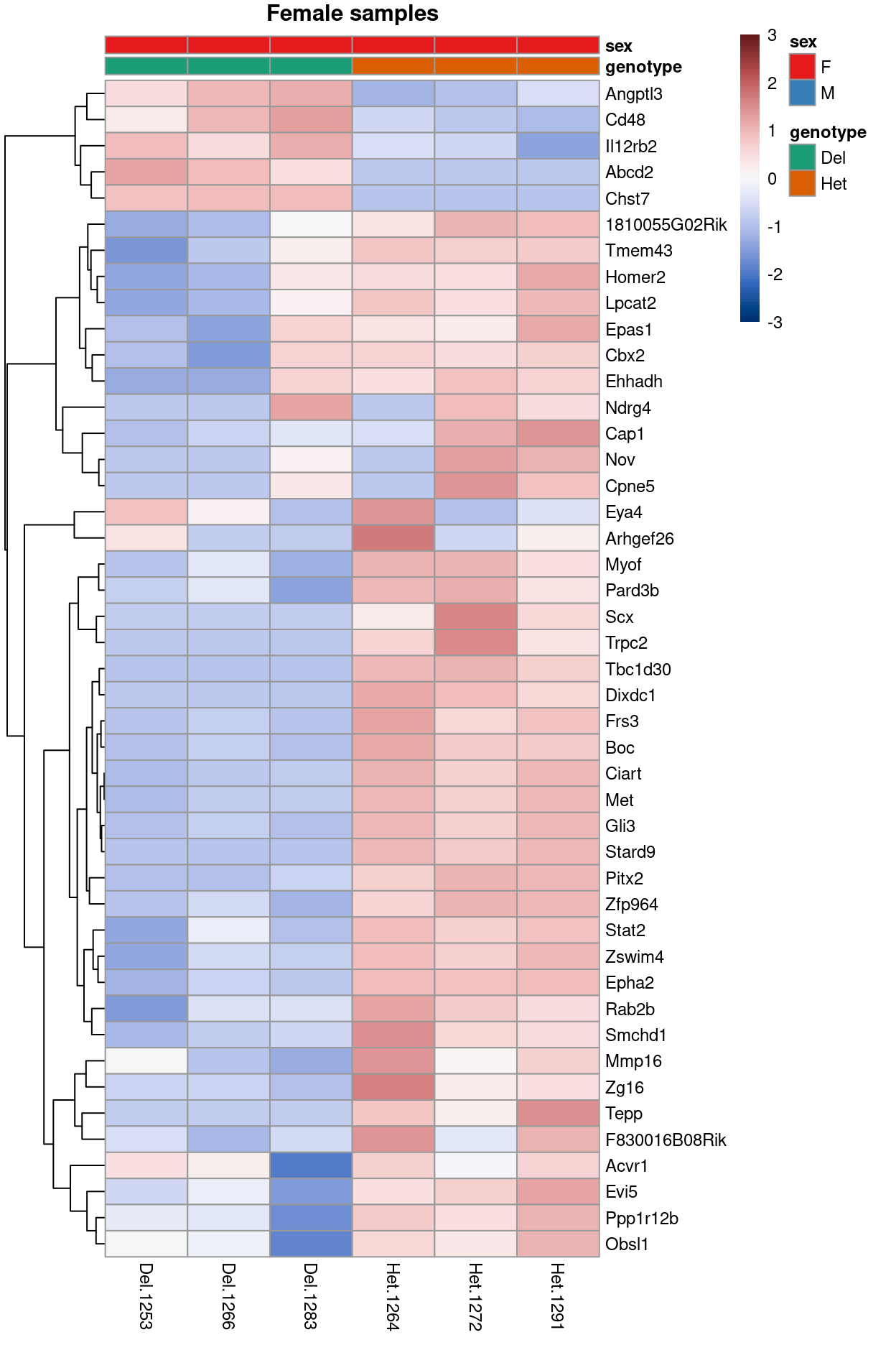
Figure 15: Heatmap of upper-quartile-normalzied logCPM values for the DEGs.

Show code

dev.off()
dir.create(here("output/figures/paper"))
pdf(here("output/figures/paper/heatmap.pdf"), height = 9, width = 6)
par(mfrow = c(1, 1))
heatmapForPaper()
dev.off()

Gene set tests

Gene set testing is commonly used to interpret the differential expression results in a biological context. Here we apply various gene set tests to the DEG lists.

goana

We use the goana() function from the limma R/Bioconductor package to test for over-representation of gene ontology (GO) terms in each DEG list.

Show code

list_of_go <- lapply(colnames(yf_contrast), function(j) {
  dgelrt <- glmLRT(yf_dgeglm, contrast = yf_contrast[, j])
  
  go <- goana(
    de = dgelrt,
    geneid = sapply(strsplit(dgelrt$genes$NCBI.ENTREZID, "; "), "[[", 1),
    species = "Mm")
  gzout <- gzfile(
    description = file.path(
      outdir, 
      "aggregated_tech_reps.females.goana.csv.gz"),
    open = "wb")
  write.csv(
    topGO(go, number = Inf),
    gzout,
    row.names = TRUE)
  close(gzout)
  go
})
names(list_of_go) <- colnames(yf_contrast)

CSV files of the results are available from output/DEGs/reads/.

An example of the results are shown below.

Show code

topGO(list_of_go[[1]]) %>%
  knitr::kable(
    caption = '`goana()` produces a table with a row for each GO term and the following columns: **Term** (GO term); **Ont** (ontology that the GO term belongs to. Possible values are "BP", "CC" and "MF"); **N** (number of genes in the GO term); **Up** (number of up-regulated differentially expressed genes); **Down** (number of down-regulated differentially expressed genes); **P.Up** (p-value for over-representation of GO term in up-regulated genes); **P.Down** (p-value for over-representation of GO term in down-regulated genes)')

Table 12: goana() produces a table with a row for each GO term and the following columns: Term (GO term); Ont (ontology that the GO term belongs to. Possible values are “BP,” “CC” and “MF”); N (number of genes in the GO term); Up (number of up-regulated differentially expressed genes); Down (number of down-regulated differentially expressed genes); P.Up (p-value for over-representation of GO term in up-regulated genes); P.Down (p-value for over-representation of GO term in down-regulated genes)

	Term	Ont	N	Up	Down	P.Up	P.Down
GO:0009653	anatomical structure morphogenesis	BP	1565	1	19	0.5223220	0.0000003
GO:0048562	embryonic organ morphogenesis	BP	156	0	6	1.0000000	0.0000156
GO:0050996	positive regulation of lipid catabolic process	BP	15	2	0	0.0000161	1.0000000
GO:0048754	branching morphogenesis of an epithelial tube	BP	93	0	5	1.0000000	0.0000171
GO:0048568	embryonic organ development	BP	268	0	7	1.0000000	0.0000353
GO:0035993	deltoid tuberosity development	BP	3	0	2	1.0000000	0.0000360
GO:0061138	morphogenesis of a branching epithelium	BP	110	0	5	1.0000000	0.0000385
GO:0007166	cell surface receptor signaling pathway	BP	1413	1	15	0.4842227	0.0000454
GO:0001763	morphogenesis of a branching structure	BP	118	0	5	1.0000000	0.0000539
GO:0061061	muscle structure development	BP	393	0	8	1.0000000	0.0000544
GO:0009887	animal organ morphogenesis	BP	533	0	9	1.0000000	0.0000746
GO:0014902	myotube differentiation	BP	68	0	4	1.0000000	0.0000902
GO:0050994	regulation of lipid catabolic process	BP	35	2	0	0.0000911	1.0000000
GO:0090596	sensory organ morphogenesis	BP	137	0	5	1.0000000	0.0001095
GO:0048593	camera-type eye morphogenesis	BP	72	0	4	1.0000000	0.0001128
GO:0090630	activation of GTPase activity	BP	75	0	4	1.0000000	0.0001322
GO:0019199	transmembrane receptor protein kinase activity	MF	30	0	3	1.0000000	0.0001523
GO:0048557	embryonic digestive tract morphogenesis	BP	6	0	2	1.0000000	0.0001786
GO:0003170	heart valve development	BP	32	0	3	1.0000000	0.0001852
GO:0001707	mesoderm formation	BP	33	0	3	1.0000000	0.0002032

kegga

We use the kegga() function from the limma R/Bioconductor package to test for over-representation of KEGG pathways in each DEG list.

Show code

list_of_kegg <- lapply(colnames(yf_contrast), function(j) {
  dgelrt <- glmLRT(yf_dgeglm, contrast = yf_contrast[, j])
  
  kegg <- kegga(
    de = dgelrt,
    geneid = sapply(strsplit(dgelrt$genes$NCBI.ENTREZID, "; "), "[[", 1),
    species = "Mm")
  gzout <- gzfile(
    description = file.path(
      outdir,
      "aggregated_tech_reps.females.kegga.csv.gz"),
    open = "wb")
  write.csv(
    topKEGG(kegg, number = Inf),
    gzout,
    row.names = TRUE)
  close(gzout)
  kegg
})
names(list_of_kegg) <- colnames(yf_contrast)

CSV files of the results are available from output/DEGs/reads/.

An example of the results are shown below.

Show code

topKEGG(list_of_kegg[[1]]) %>%
  knitr::kable(
    caption = '`kegga()` produces a table with a row for each KEGG pathway ID and the following columns: **Pathway** (KEGG pathway); **N** (number of genes in the GO term); **Up** (number of up-regulated differentially expressed genes); **Down** (number of down-regulated differentially expressed genes); **P.Up** (p-value for over-representation of KEGG pathway in up-regulated genes); **P.Down** (p-value for over-representation of KEGG pathway in down-regulated genes)')

Table 13: kegga() produces a table with a row for each KEGG pathway ID and the following columns: Pathway (KEGG pathway); N (number of genes in the GO term); Up (number of up-regulated differentially expressed genes); Down (number of down-regulated differentially expressed genes); P.Up (p-value for over-representation of KEGG pathway in up-regulated genes); P.Down (p-value for over-representation of KEGG pathway in down-regulated genes)

	Pathway	N	Up	Down	P.Up	P.Down
path:mmu04360	Axon guidance	109	0	3	1.0000000	0.0065037
path:mmu00532	Glycosaminoglycan biosynthesis - chondroitin sulfate / dermatan sulfate	15	1	0	0.0065651	1.0000000
path:mmu04340	Hedgehog signaling pathway	42	0	2	1.0000000	0.0094658
path:mmu02010	ABC transporters	25	1	0	0.0109226	1.0000000
path:mmu04979	Cholesterol metabolism	29	1	0	0.0126614	1.0000000
path:mmu04350	TGF-beta signaling pathway	55	0	2	1.0000000	0.0158649
path:mmu05321	Inflammatory bowel disease	38	1	0	0.0165646	1.0000000
path:mmu05100	Bacterial invasion of epithelial cells	61	0	2	1.0000000	0.0192945
path:mmu05211	Renal cell carcinoma	62	0	2	1.0000000	0.0198939
path:mmu04658	Th1 and Th2 cell differentiation	65	1	0	0.0282002	1.0000000
path:mmu04650	Natural killer cell mediated cytotoxicity	67	1	0	0.0290577	1.0000000
path:mmu04146	Peroxisome	67	1	1	0.0290577	0.2104325
path:mmu05200	Pathways in cancer	352	1	4	0.1452135	0.0341319
path:mmu04630	JAK-STAT signaling pathway	94	1	1	0.0405748	0.2824260
path:mmu04060	Cytokine-cytokine receptor interaction	96	1	1	0.0414235	0.2874965
path:mmu00650	Butanoate metabolism	16	0	1	1.0000000	0.0547407
path:mmu00410	beta-Alanine metabolism	20	0	1	1.0000000	0.0679626
path:mmu00380	Tryptophan metabolism	21	0	1	1.0000000	0.0712398
path:mmu04510	Focal adhesion	127	0	2	1.0000000	0.0730508
path:mmu05206	MicroRNAs in cancer	131	0	2	1.0000000	0.0770741

camera with MSigDB gene sets

We use the camera() function from the limma R/Bioconductor package to test whether a set of genes is highly ranked relative to other genes in terms of differential expression, accounting for inter-gene correlation. Specifically, we test using gene sets from MSigDB, namely:

We download these gene sets from http://bioinf.wehi.edu.au/MSigDB/index.html

• H: hallmark gene sets are coherently expressed signatures derived by aggregating many MSigDB gene sets to represent well-defined biological states or processes.
• C2: curated gene sets from online pathway databases, publications in PubMed, and knowledge of domain experts.

Show code

yf_idx <- ids2indices(
  msigdb, 
  id = sapply(strsplit(yf$genes$NCBI.ENTREZID, "; "), "[[", 1))
list_of_camera <- lapply(colnames(yf_contrast), function(j) {
  cam <- camera(
    y = yf, 
    index = yf_idx,
    design = yf_design, 
    contrast = yf_contrast[, j])
  gzout <- gzfile(
    description = file.path(
      outdir, 
      "aggregated_tech_reps.females.camera.csv.gz"),
    open = "wb")
  write.csv(
    cam,
    gzout,
    row.names = TRUE)
  close(gzout)
  cam
})
names(list_of_camera) <- colnames(yf_contrast)

CSV files of the results are available from output/DEGs/reads.

An example of the results are shown below.

Show code

head(list_of_camera[[1]]) %>%
  knitr::kable(
    caption = '`camera()` produces a table with a row for each gene set (prepended by which MSigDB collection it comes from) and the following columns: **NGenes** (number of genes in set); **Direction** (direction of change); **PValue** (two-tailed p-value); **FDR** (Benjamini and Hochberg FDR adjusted p-value).')

Table 14: camera() produces a table with a row for each gene set (prepended by which MSigDB collection it comes from) and the following columns: NGenes (number of genes in set); Direction (direction of change); PValue (two-tailed p-value); FDR (Benjamini and Hochberg FDR adjusted p-value).

	NGenes	Direction	PValue	FDR
C2.KEGG_RIBOSOME	102	Up	0	1.0e-07
C2.REACTOME_EUKARYOTIC_TRANSLATION_ELONGATION	107	Up	0	1.0e-07
C2.REACTOME_RESPONSE_OF_EIF2AK4_GCN2_TO_AMINO_ACID_DEFICIENCY	115	Up	0	9.0e-07
C2.REACTOME_RESPIRATORY_ELECTRON_TRANSPORT_ATP_SYNTHESIS_BY_CHEMIOSMOTIC_COUPLING_AND_HEAT_PRODUCTION_BY_UNCOUPLING_PROTEINS	121	Up	0	1.3e-06
C2.REACTOME_EUKARYOTIC_TRANSLATION_INITIATION	139	Up	0	1.3e-06
C2.REACTOME_SRP_DEPENDENT_COTRANSLATIONAL_PROTEIN_TARGETING_TO_MEMBRANE	130	Up	0	1.9e-06

Sarah’s gene lists

Show code

yf_X <- yf$genes$ENSEMBL.SEQNAME == "X"
yf_protocadherin <- grepl("Pcdh", rownames(yf))
yf_pw <- rownames(yf) %in% c("Ndn", "Mkrn3", "Peg12")
yf_male <- male_het_vs_del[
  male_het_vs_del$FDR < 0.05,
  c("ENSEMBL.SYMBOL", "logFC")]
yf_female <- male_het_vs_del[
  female_het_vs_del$FDR < 0.05,
  c("ENSEMBL.SYMBOL", "logFC")]
yf_sun <- sun_2014[, c("geneSymbol", "log2FC")]
yf_chambers <- chambers_2007[, c("Gene Symbol", "Fold Difference")]
yf_chambers$logFC <- log2(yf_chambers$`Fold Difference`)
yf_chambers$`Fold Difference` <- NULL
yf_chambers <- yf_chambers[!is.na(yf_chambers$`Gene Symbol`), ]
yf_chambers <- yf_chambers[!duplicated(yf_chambers$`Gene Symbol`), ]
yf_gazit <- gazit_2013[, c("Symbol"), drop = FALSE]
yf_gazit$Symbol <- paste(
  substring(yf_gazit$Symbol, 1, 1), 
  tolower(substring(yf_gazit$Symbol, 2)),
  sep = "")
yf_gazit$logFC <- 1
yf_chambers_gazit <- data.frame(
  Symbol = c(yf_chambers$`Gene Symbol`, yf_gazit$Symbol),
  logFC = c(yf_chambers$logFC, yf_gazit$logFC))
yf_chambers_gazit <- yf_chambers_gazit[!duplicated(yf_chambers_gazit$Symbol), ]
yf_venezia_proliferation <- rownames(yf) %in% venezia_proliferation$Gene.Symbol
yf_venezia_quiescence <- rownames(yf) %in% venezia_quiescence$Gene.Symbol

yf_index <- list(
  `X-linked` = yf_X,
  Protocadherin = yf_protocadherin,
  `Prader-Willi` = yf_pw,
  `Male: Het vs. Del` = yf_male,
  `Female: Het vs. Del` = yf_female,
  `Sun (2014)` = yf_sun,
  `Chambers (2007)` = yf_chambers,
  `Gazit (2013)` = yf_gazit,
  `Chambers (2007) & Gazit (2013)` = yf_chambers_gazit,
  `Proliferation Group Venezia (2004)` = yf_venezia_proliferation,
  `Quiescence Group Venezia (2004)` = yf_venezia_quiescence)

Sarah requested testing a number of gene sets (see Gene sets).

We use the fry() function from the edgeR R/Bioconductor package to perform a self-contained gene set test against the null hypothesis that none of the genes in the set are differentially expressed.

Show code

fry(
  yf, 
  index = yf_index, 
  design = yf_design,
  contrast = yf_contrast,
  sort = "none") %>%
    knitr::kable(
      caption = "Results of applying `fry()` to the RNA-seq differential expression results using the supplied gene sets. A significant 'Up' P-value means that the differential expression results found in the RNA-seq data are positively correlated with the expression signature from the corresponding gene set. Conversely, a significant 'Down' P-value means that the differential expression log-fold-changes are negatively correlated with the expression signature from the corresponding gene set. A significant 'Mixed' P-value means that the genes in the set tend to be differentially expressed without regard for direction.")

Table 15: Results of applying fry() to the RNA-seq differential expression results using the supplied gene sets. A significant ‘Up’ P-value means that the differential expression results found in the RNA-seq data are positively correlated with the expression signature from the corresponding gene set. Conversely, a significant ‘Down’ P-value means that the differential expression log-fold-changes are negatively correlated with the expression signature from the corresponding gene set. A significant ‘Mixed’ P-value means that the genes in the set tend to be differentially expressed without regard for direction.

	NGenes	Direction	PValue	FDR	PValue.Mixed	FDR.Mixed
X-linked	385	Down	0.7932572	0.8725829	0.0009255	0.0101804
Protocadherin	6	Up	0.3450358	0.5421992	0.5544190	0.7140077
Prader-Willi	3	Up	0.5275007	0.7253135	0.8358759	0.8358759
Male: Het vs. Del	7	Up	0.6811221	0.8324826	0.6306529	0.7140077
Female: Het vs. Del	16	Up	0.9166151	0.9166151	0.6490979	0.7140077
Sun (2014)	1986	Down	0.1441139	0.2642088	0.0025603	0.0140817
Chambers (2007)	204	Down	0.0110643	0.0961422	0.0219285	0.0482426
Gazit (2013)	248	Down	0.0573814	0.1577988	0.0189400	0.0482426
Chambers (2007) & Gazit (2013)	399	Down	0.0174804	0.0961422	0.0210045	0.0482426
Proliferation Group Venezia (2004)	365	Up	0.0531114	0.1577988	0.0462182	0.0847334
Quiescence Group Venezia (2004)	381	Down	0.0727634	0.1600795	0.1389243	0.2183096

Show code

geneSetTestFiguresForPaper <- function() {
  for (n in names(yf_index)) {
    if (is.data.frame(yf_index[[n]])) {
      yf_status <- rep(0, nrow(yf_dgelrt))
      yf_status[rownames(yf) %in% yf_index[[n]][, 1]] <-
        sign(yf_index[[n]][yf_index[[n]][, 1] %in% rownames(yf), 2])
      plotMD(
        yf_dgelrt,
        status = yf_status,
        hl.col = c("red", "blue"),
        legend = "bottomright",
        main = n)
      abline(h = 0, col = "darkgrey")
    } else {
      yf_status <- rep("Other", nrow(yf_dgelrt))
      yf_status[yf_index[[n]]] <- n
      plotMD(
        yf_dgelrt,
        status = yf_status,
        values = n,
        hl.col = "red",
        legend = "bottomright",
        main = n)
      abline(h = 0, col = "darkgrey")
    }
    
    if (is.data.frame(yf_index[[n]])) {
      barcodeplot(
        yf_dgelrt$table$logFC,
        rownames(yf) %in% yf_index[[n]][, 1],
        gene.weights = yf_index[[n]][
          yf_index[[n]][, 1] %in% rownames(yf), 2],
        main = n)
    } else {
      barcodeplot(
        yf_dgelrt$table$logFC,
        yf_index[[n]],
        main = n)
    }
  }
}

Show code

par(mfrow = c(length(yf_index), 2))
geneSetTestFiguresForPaper()  

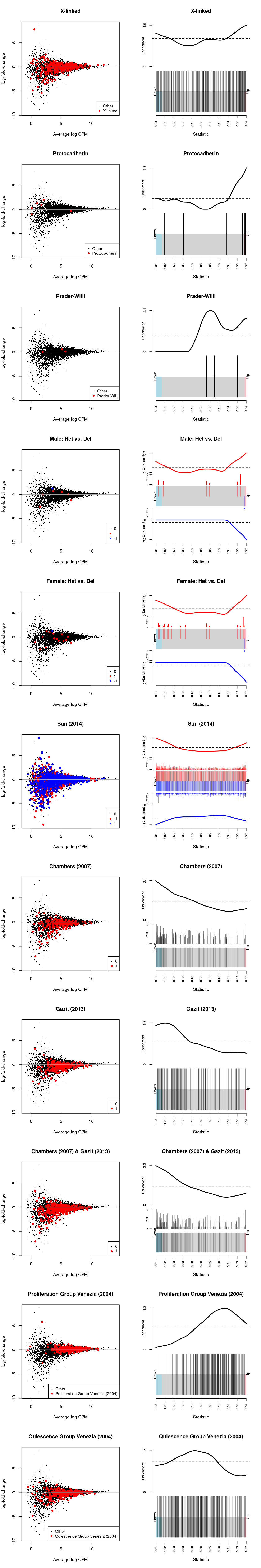
Figure 16: MD-plot and barcode plot of genes in supplied gene sets. Directional gene sets have (1) MD plot points coloured according to the statistical significance of the gene in the gene set (2) barcode plot ‘weights’ given by the logFC of the gene in the gene set. For the barcode plot, genes are represented by bars and are ranked from left to right by increasing log-fold change. This forms the barcode-like pattern. The line (or worm) above the barcode shows the relative local enrichment of the vertical bars in each part of the plot. The dotted horizontal line indicates neutral enrichment; the worm above the dotted line shows enrichment while the worm below the dotted line shows depletion.

A PDF version of these figures are available in output/figures/paper/gene_set_tests.pdf.

Show code

dir.create(here("output/figures/paper"))
pdf(here("output/figures/paper/gene_set_tests.pdf"), height = 6, width = 6)
par(mfrow = c(1, 1))
geneSetTestFiguresForPaper()
dev.off()

Session info

The analysis and this document were prepared using the following software (click triangle to expand)

Show code

sessioninfo::session_info()

─ Session info ─────────────────────────────────────────────────────
 setting  value                       
 version  R version 4.0.3 (2020-10-10)
 os       CentOS Linux 7 (Core)       
 system   x86_64, linux-gnu           
 ui       X11                         
 language (EN)                        
 collate  en_US.UTF-8                 
 ctype    en_US.UTF-8                 
 tz       Australia/Melbourne         
 date     2021-10-20                  

─ Packages ─────────────────────────────────────────────────────────
 ! package              * version  date       lib source        
 P annotate               1.68.0   2020-10-27 [?] Bioconductor  
 P AnnotationDbi          1.52.0   2020-10-27 [?] Bioconductor  
 P aroma.light            3.20.0   2020-10-27 [?] Bioconductor  
 P askpass                1.1      2019-01-13 [?] CRAN (R 4.0.0)
 P assertthat             0.2.1    2019-03-21 [?] CRAN (R 4.0.0)
 P Biobase              * 2.50.0   2020-10-27 [?] Bioconductor  
 P BiocFileCache        * 1.14.0   2020-10-27 [?] Bioconductor  
 P BiocGenerics         * 0.36.0   2020-10-27 [?] Bioconductor  
 P BiocManager            1.30.10  2019-11-16 [?] CRAN (R 4.0.0)
 P BiocParallel         * 1.24.1   2020-11-06 [?] Bioconductor  
 P BiocStyle              2.18.1   2020-11-24 [?] Bioconductor  
 P biomaRt                2.46.3   2021-02-09 [?] Bioconductor  
 P Biostrings           * 2.58.0   2020-10-27 [?] Bioconductor  
 P bit                    4.0.4    2020-08-04 [?] CRAN (R 4.0.0)
 P bit64                  4.0.5    2020-08-30 [?] CRAN (R 4.0.0)
 P bitops                 1.0-6    2013-08-17 [?] CRAN (R 4.0.0)
 P blob                   1.2.1    2020-01-20 [?] CRAN (R 4.0.0)
 P cachem                 1.0.4    2021-02-13 [?] CRAN (R 4.0.3)
 P cellranger             1.1.0    2016-07-27 [?] CRAN (R 4.0.0)
 P cli                    2.3.1    2021-02-23 [?] CRAN (R 4.0.3)
 P colorspace             2.0-0    2020-11-11 [?] CRAN (R 4.0.3)
 P cowplot              * 1.1.1    2020-12-30 [?] CRAN (R 4.0.3)
 P crayon                 1.4.1    2021-02-08 [?] CRAN (R 4.0.3)
 P crosstalk              1.1.1    2021-01-12 [?] CRAN (R 4.0.3)
 P curl                   4.3      2019-12-02 [?] CRAN (R 4.0.0)
 P data.table             1.14.0   2021-02-21 [?] CRAN (R 4.0.3)
 P DBI                    1.1.1    2021-01-15 [?] CRAN (R 4.0.3)
 P dbplyr               * 2.1.0    2021-02-03 [?] CRAN (R 4.0.3)
 P DelayedArray           0.16.1   2021-01-22 [?] Bioconductor  
 P DESeq2                 1.30.1   2021-02-19 [?] Bioconductor  
 P digest                 0.6.27   2020-10-24 [?] CRAN (R 4.0.2)
 P distill                1.2      2021-01-13 [?] CRAN (R 4.0.3)
 P downlit                0.2.1    2020-11-04 [?] CRAN (R 4.0.3)
 P dplyr                  1.0.4    2021-02-02 [?] CRAN (R 4.0.3)
 P DT                     0.17     2021-01-06 [?] CRAN (R 4.0.3)
 P EDASeq               * 2.24.0   2020-10-27 [?] Bioconductor  
 P edgeR                * 3.32.1   2021-01-14 [?] Bioconductor  
 P ellipsis               0.3.1    2020-05-15 [?] CRAN (R 4.0.0)
 P evaluate               0.14     2019-05-28 [?] CRAN (R 4.0.0)
 P fansi                  0.4.2    2021-01-15 [?] CRAN (R 4.0.3)
 P farver                 2.0.3    2020-01-16 [?] CRAN (R 4.0.0)
 P fastmap                1.1.0    2021-01-25 [?] CRAN (R 4.0.3)
 P genefilter             1.72.1   2021-01-21 [?] Bioconductor  
 P geneplotter            1.68.0   2020-10-27 [?] Bioconductor  
 P generics               0.1.0    2020-10-31 [?] CRAN (R 4.0.3)
 P GenomeInfoDb         * 1.26.2   2020-12-08 [?] Bioconductor  
 P GenomeInfoDbData       1.2.4    2020-10-20 [?] Bioconductor  
 P GenomicAlignments    * 1.26.0   2020-10-27 [?] Bioconductor  
 P GenomicFeatures        1.42.1   2020-11-12 [?] Bioconductor  
 P GenomicRanges        * 1.42.0   2020-10-27 [?] Bioconductor  
 P ggplot2              * 3.3.3    2020-12-30 [?] CRAN (R 4.0.3)
 P ggrepel              * 0.9.1    2021-01-15 [?] CRAN (R 4.0.3)
 P Glimma               * 2.0.0    2020-10-27 [?] Bioconductor  
 P glue                   1.4.2    2020-08-27 [?] CRAN (R 4.0.0)
 P GO.db                  3.12.1   2020-11-04 [?] Bioconductor  
 P gtable                 0.3.0    2019-03-25 [?] CRAN (R 4.0.0)
 P here                 * 1.0.1    2020-12-13 [?] CRAN (R 4.0.3)
 P highr                  0.8      2019-03-20 [?] CRAN (R 4.0.0)
 P hms                    1.0.0    2021-01-13 [?] CRAN (R 4.0.3)
 P htmltools              0.5.1.1  2021-01-22 [?] CRAN (R 4.0.3)
 P htmlwidgets            1.5.3    2020-12-10 [?] CRAN (R 4.0.3)
 P httr                   1.4.2    2020-07-20 [?] CRAN (R 4.0.0)
 P hwriter                1.3.2    2014-09-10 [?] CRAN (R 4.0.0)
 P IRanges              * 2.24.1   2020-12-12 [?] Bioconductor  
 P jpeg                   0.1-8.1  2019-10-24 [?] CRAN (R 4.0.0)
 P jsonlite               1.7.2    2020-12-09 [?] CRAN (R 4.0.3)
 P knitr                  1.31     2021-01-27 [?] CRAN (R 4.0.3)
 P labeling               0.4.2    2020-10-20 [?] CRAN (R 4.0.0)
 P lattice                0.20-41  2020-04-02 [3] CRAN (R 4.0.3)
 P latticeExtra           0.6-29   2019-12-19 [?] CRAN (R 4.0.0)
 P lifecycle              1.0.0    2021-02-15 [?] CRAN (R 4.0.3)
 P limma                * 3.46.0   2020-10-27 [?] Bioconductor  
 P locfit                 1.5-9.4  2020-03-25 [?] CRAN (R 4.0.0)
 P magrittr             * 2.0.1    2020-11-17 [?] CRAN (R 4.0.3)
 P MASS                   7.3-53   2020-09-09 [3] CRAN (R 4.0.3)
 P Matrix                 1.2-18   2019-11-27 [3] CRAN (R 4.0.3)
 P MatrixGenerics       * 1.2.1    2021-01-30 [?] Bioconductor  
 P matrixStats          * 0.58.0   2021-01-29 [?] CRAN (R 4.0.3)
 P memoise                2.0.0    2021-01-26 [?] CRAN (R 4.0.3)
 P munsell                0.5.0    2018-06-12 [?] CRAN (R 4.0.0)
 P openssl                1.4.3    2020-09-18 [?] CRAN (R 4.0.2)
 P org.Mm.eg.db           3.12.0   2020-10-20 [?] Bioconductor  
 P patchwork            * 1.1.1    2020-12-17 [?] CRAN (R 4.0.3)
 P pheatmap             * 1.0.12   2019-01-04 [?] CRAN (R 4.0.0)
 P pillar                 1.5.0    2021-02-22 [?] CRAN (R 4.0.3)
 P pkgconfig              2.0.3    2019-09-22 [?] CRAN (R 4.0.0)
 P png                    0.1-7    2013-12-03 [?] CRAN (R 4.0.0)
 P prettyunits            1.1.1    2020-01-24 [?] CRAN (R 4.0.0)
 P progress               1.2.2    2019-05-16 [?] CRAN (R 4.0.0)
 P purrr                  0.3.4    2020-04-17 [?] CRAN (R 4.0.0)
 P R.methodsS3            1.8.1    2020-08-26 [?] CRAN (R 4.0.0)
 P R.oo                   1.24.0   2020-08-26 [?] CRAN (R 4.0.0)
 P R.utils                2.10.1   2020-08-26 [?] CRAN (R 4.0.0)
 P R6                     2.5.0    2020-10-28 [?] CRAN (R 4.0.2)
 P rappdirs               0.3.3    2021-01-31 [?] CRAN (R 4.0.3)
 P RColorBrewer           1.1-2    2014-12-07 [?] CRAN (R 4.0.0)
 P Rcpp                   1.0.6    2021-01-15 [?] CRAN (R 4.0.3)
 P RCurl                  1.98-1.2 2020-04-18 [?] CRAN (R 4.0.0)
 P readxl               * 1.3.1    2019-03-13 [?] CRAN (R 4.0.0)
 P rematch                1.0.1    2016-04-21 [?] CRAN (R 4.0.0)
 P rlang                  0.4.10   2020-12-30 [?] CRAN (R 4.0.3)
 P rmarkdown              2.11     2021-09-14 [?] CRAN (R 4.0.0)
 P rprojroot              2.0.2    2020-11-15 [?] CRAN (R 4.0.3)
 P Rsamtools            * 2.6.0    2020-10-27 [?] Bioconductor  
 P RSQLite                2.2.3    2021-01-24 [?] CRAN (R 4.0.3)
 P rtracklayer            1.50.0   2020-10-27 [?] Bioconductor  
 P RUVSeq               * 1.24.0   2020-10-27 [?] Bioconductor  
 P S4Vectors            * 0.28.1   2020-12-09 [?] Bioconductor  
 P scales                 1.1.1    2020-05-11 [?] CRAN (R 4.0.0)
 P sessioninfo            1.1.1    2018-11-05 [?] CRAN (R 4.0.0)
 P ShortRead            * 1.48.0   2020-10-27 [?] Bioconductor  
 P SingleCellExperiment * 1.12.0   2020-10-27 [?] Bioconductor  
 P stringi                1.5.3    2020-09-09 [?] CRAN (R 4.0.0)
 P stringr                1.4.0    2019-02-10 [?] CRAN (R 4.0.0)
 P SummarizedExperiment * 1.20.0   2020-10-27 [?] Bioconductor  
 P survival               3.2-7    2020-09-28 [3] CRAN (R 4.0.3)
 P tibble                 3.0.6    2021-01-29 [?] CRAN (R 4.0.3)
 P tidyselect             1.1.0    2020-05-11 [?] CRAN (R 4.0.0)
 P utf8                   1.1.4    2018-05-24 [?] CRAN (R 4.0.0)
 P vctrs                  0.3.6    2020-12-17 [?] CRAN (R 4.0.3)
 P viridisLite            0.3.0    2018-02-01 [?] CRAN (R 4.0.0)
 P withr                  2.4.1    2021-01-26 [?] CRAN (R 4.0.3)
 P xfun                   0.26     2021-09-14 [?] CRAN (R 4.0.0)
 P XML                    3.99-0.5 2020-07-23 [?] CRAN (R 4.0.0)
 P xml2                   1.3.2    2020-04-23 [?] CRAN (R 4.0.0)
 P xtable                 1.8-4    2019-04-21 [?] CRAN (R 4.0.0)
 P XVector              * 0.30.0   2020-10-27 [?] Bioconductor  
 P yaml                   2.2.1    2020-02-01 [?] CRAN (R 4.0.0)
 P zlibbioc               1.36.0   2020-10-27 [?] Bioconductor  

[1] /stornext/Projects/score/Analyses/C086_Kinkel/renv/library/R-4.0/x86_64-pc-linux-gnu
[2] /tmp/RtmpfgojZ6/renv-system-library
[3] /stornext/System/data/apps/R/R-4.0.3/lib64/R/library

 P ── Loaded and on-disk path mismatch.

---

1. Details of RUVs parameters are given separately for each analysis.↩︎

2. see [docs/C086_Kinkel.male_B_cells.multi-sample_comparisons.html(../docs/C086_Kinkel.male_B_cells.multi-sample_comparisons.html)]↩︎

3. see [docs/C086_Kinkel.female_B_cells.multi-sample_comparisons.html(../docs/C086_Kinkel.female_B_cells.multi-sample_comparisons.html)]↩︎

4. My understanding of this terms translates as ‘upregulated DEGs.’↩︎