Table of Contents
Motivation
scRNA-seq datasets may include cells that are not relevant to the study, even after the initial quality control, which we don’t want to include in downstream analyses. In this section aim to filter out these ‘unwanted’ cells and retain only the ‘biologically relevant’ cells. Examples of unwanted cells include:
- Cells with ‘reasonable’ QC metrics, but that are transcriptomically distinct from the majority of cells in the dataset
- Cells of unwanted cell types, such as those that might sneak through a FACS or magnetic bead enrichment sample preparation
Once we are confident that we have selected the biologically relevant cells, we will perform data integration (if necessary) and a further round of clustering in preparation for downstream analysis.
The removal of unwanted cells is an iterative process where at each step we:
- Identify cluster(s) enriched for unwanted cells. The exact criteria used to define ‘unwanted’ will depend on the type of cells we are trying to identify at each step.
- Perform diagnostic checks to ensure we aren’t discarding biologically relevant cells.
- Remove the unwanted cells.
- Re-process the remaining cells.
- Identify HVGs.
- Perform dimensionality reduction (PCA and UMAP).
- Cluster cells.
Clustering is a critical component of this process, so we discuss it in further detail in the next subsection.
Clustering
Clustering is an unsupervised learning procedure that is used in scRNA-seq data analysis to empirically define groups of cells with similar expression profiles. Its primary purpose is to summarize the data in a digestible format for human interpretation. This allows us to describe population heterogeneity in terms of discrete labels that are easily understood, rather than attempting to comprehend the high-dimensional manifold on which the cells truly reside. Clustering is thus a critical step for extracting biological insights from scRNA-seq data.
Clustering calculations are usually performed using the top PCs to take advantage of data compression and denoising1.
Clusters vs. cell types
It is worth stressing the distinction between clusters and cell types. The former is an empirical construct while the latter is a biological truth (albeit a vaguely defined one). For this reason, questions like “what is the true number of clusters?” are usually meaningless. We can define as many clusters as we like, with whatever algorithm we like - each clustering will represent its own partitioning of the high-dimensional expression space, and is as “real” as any other clustering.
A more relevant question is “how well do the clusters approximate the cell types?” Unfortunately, this is difficult to answer given the context-dependent interpretation of biological truth. Some analysts will be satisfied with resolution of the major cell types; other analysts may want resolution of subtypes; and others still may require resolution of different states (e.g., metabolic activity, stress) within those subtypes. Two clusterings can also be highly inconsistent yet both valid, simply partitioning the cells based on different aspects of biology. Indeed, asking for an unqualified “best” clustering is akin to asking for the best magnification on a microscope without any context.
It is helpful to realize that clustering, like a microscope, is simply a tool to explore the data. We can zoom in and out by changing the resolution of the clustering parameters, and we can experiment with different clustering algorithms to obtain alternative perspectives of the data. This iterative approach is entirely permissible for data exploration, which constitutes the majority of all scRNA-seq data analysis.
Graph-based clustering
We build a shared nearest neighbour graph (Xu and Su 2015) and use the Louvain algorithm to identify clusters. We would build the graph using the principal components.
Preparing the data
We start from the preprocessed SingleCellExperiment object created in ‘Preprocessing the Grant (C075) retinal epithelial cells data set’.
Initial clustering
There are 8 clusters detected, shown on the UMAP plot Figure 1 and broken down by experimental factors in Figure 2.
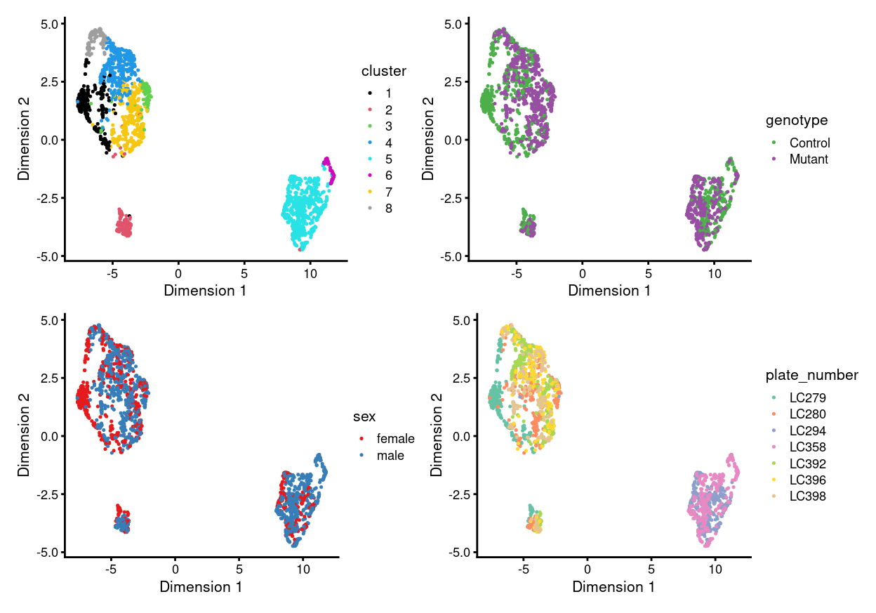
Figure 1: UMAP plot, where each point represents a cell and is coloured according to the legend.
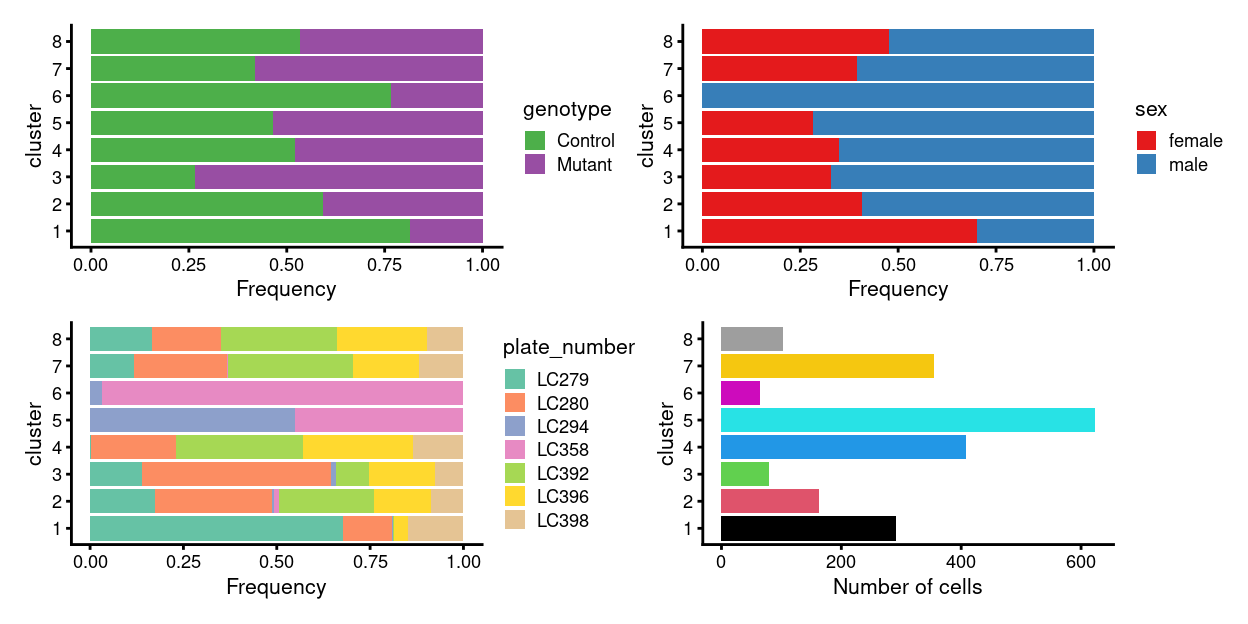
Figure 2: Breakdown of clusters by experimental factors.
Notably:
- Some of the clusters are highly plate-specific.
Plate-specific clusters
Motivation
We have seen that cells from plates LC294 and LC358 cluster separately from the remaining plates. To try to understand what is driving the differences between cells on these two sets of plates, we perform a marker gene analysis. The results of this analysis will help us decide how to handle this issue.
Analysis
We use two sets of marker genes for this analysis:
Pre-defined marker genes
Zoe sent me a list of marker genes to help characterise the cells2.
Figure 3 is a heatmap of Zoe’s marker genes. There is evidence that some of the Stem marker genes are only expressed in plates LC294 and LC358. There is also some evidence that most of the other marker genes have lower expression in cells from plates LC294 and LC358 compared to cells from the rest of the plates.
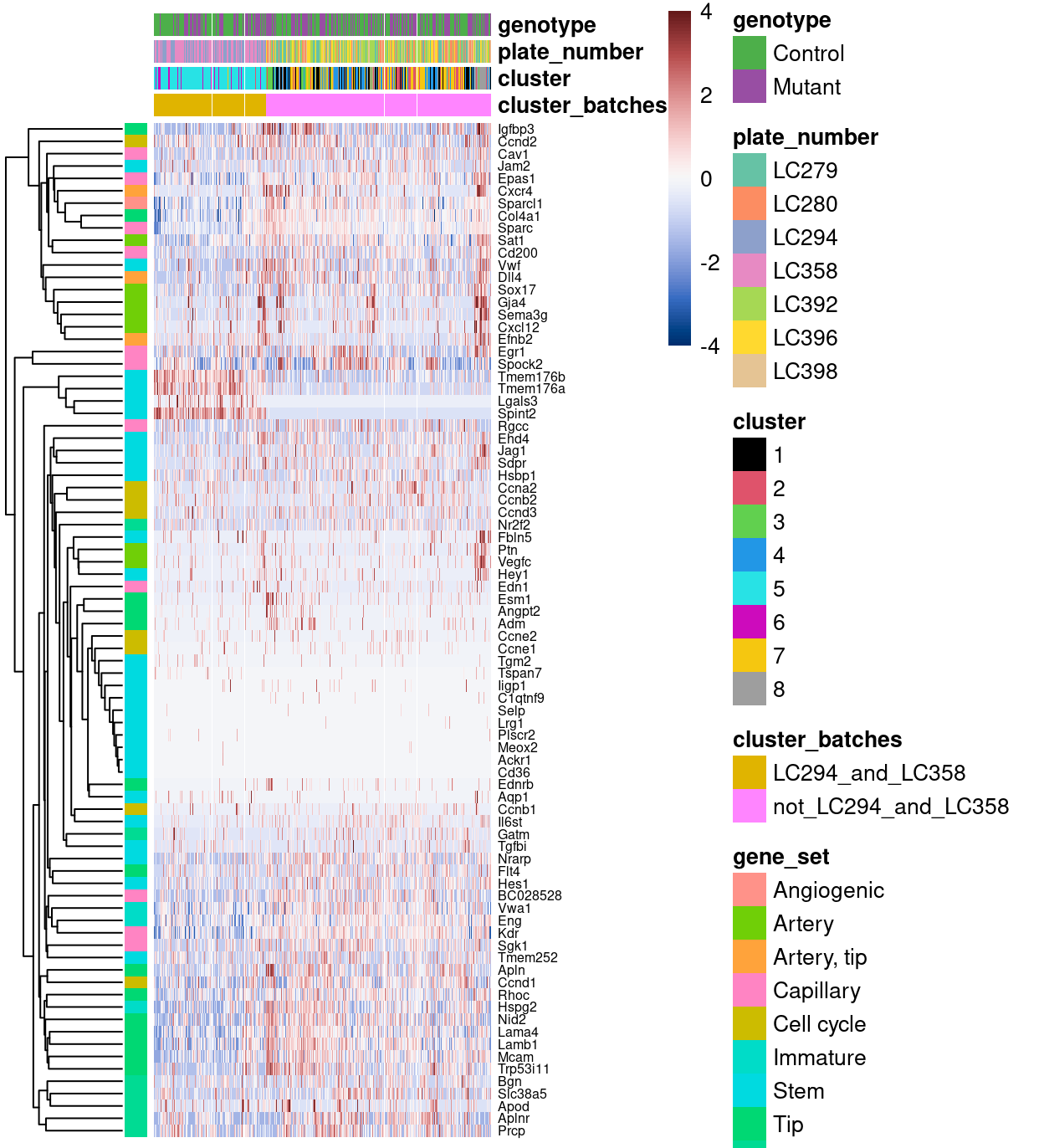
Figure 3: Heatmap of row-normalized log-expression values for Zoe’s marker genes. Each column is a sample, each row a gene. Samples have been separetely clustered within each cluster_batches.
De novo marker genes
We use a binomial test to look for genes that differ in the proportion of expressing cells from plates LC294 and LC358 compared to cells from the rest of the plates. The premise is that we want to see if there are genes that were active in one set of plates and silent in another, a potentially very serious difference between cells on the two sets of plates.
There are 3913 genes (11.6%) more frequently expressed in cells from plates LC294 and LC358 and 1797 genes (5.3%) more frequently expressed in cells from the rest of the plates (FDR \(< 0.05\)).
As an example of the information available in these gene lists, Figure 4 highlights the top-50 genes for each group of plates. What is remarkable about this figure is that it shows that there is a set of genes that are only detected in cells from plates LC294 and LC358 and that these genes are seemingly biologically relevant genes (e.g., Epcam, Cdhr5, Cdhr2). In contrast, the genes detected more frequently in the remaining plates are at least detected to some degree in plates LC294 and LC358.
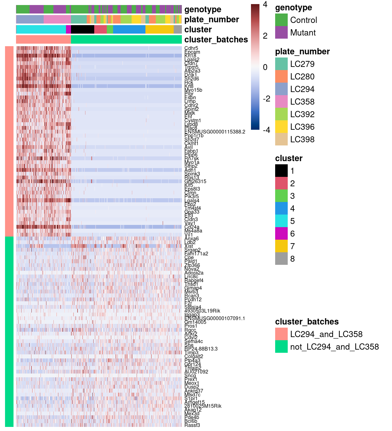
Figure 4: Heatmap of row-normalized log-expression values for selected marker genes between plates LC294 and LC358 and the rest of the plates. Each column is a sample, each row a gene.
Summary
This result was discussed with Zoe4. Zoe characterised the genes expressed exclusively by cells on plates LC294 and LC358 as being “abnormal for the cells I collected (i.e. … epithelial cell markers)” and noted that “there was nothing obviously different about the phenotype or the way that [she] prepared these samples that would explain these differences”.
Subsequent analysis identified that plates LC294 and LC358 were contaminated by RNA from a separate project (C078_Wang; see slides). SCORE was not able to determine the root cause of this contamination, but the diagnosis is clear and it was therefore decided to exclude cells from plates on LC294 and LC358 from further analysis.
Figure 5 shows that most of the remaining plates have cells from a knockout and a wildtype mouse with each pair of mice on a plate are from the same sibship5. The exception is the initial pilot plate, LC279, which has cells from a single control mouse.
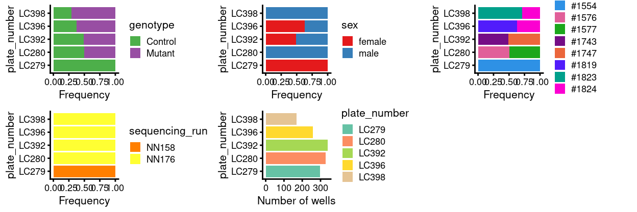
Figure 5: Breakdown of of the samples by plate.
Re-processing
There are 9 clusters detected, shown on the UMAP plot Figure 6 and broken down by experimental factors in Figure 7.
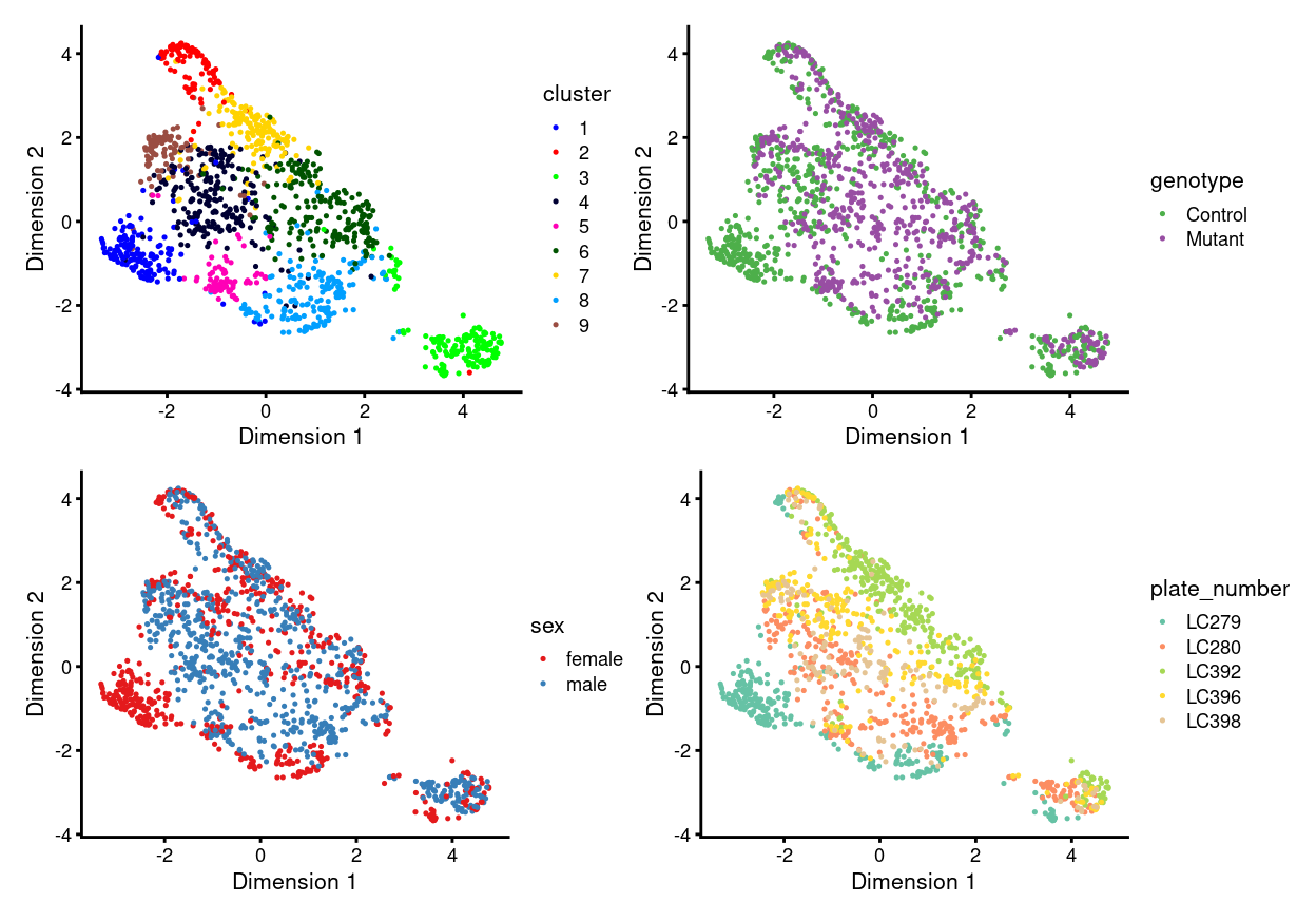
Figure 6: UMAP plot, where each point represents a cell and is coloured according to the legend.
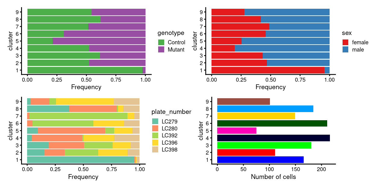
Figure 7: Breakdown of clusters by experimental factors.
Notably:
- Still, some of the clusters are highly plate-specific (i.e. potential batch effects).
We therefore proceed to Data integration to remove these plate-specific differences
Low-level within-plate contamination
Figure 8 shows that some of the cells from male samples have non-zero expression of Xist, afemale-specific gene. Notably, this only occurs in male samples on plates that also contain a female sample, which suggests that there is some low-level within-plate contamination. This within-plate contamination may be caused by well barcode swaps or by dirty tools at the time of sample dissection. Whilst somewhat concerning, it is difficult to remove this contamination and its effect is hopefully moderate compared to the wanted sources of biological variation.
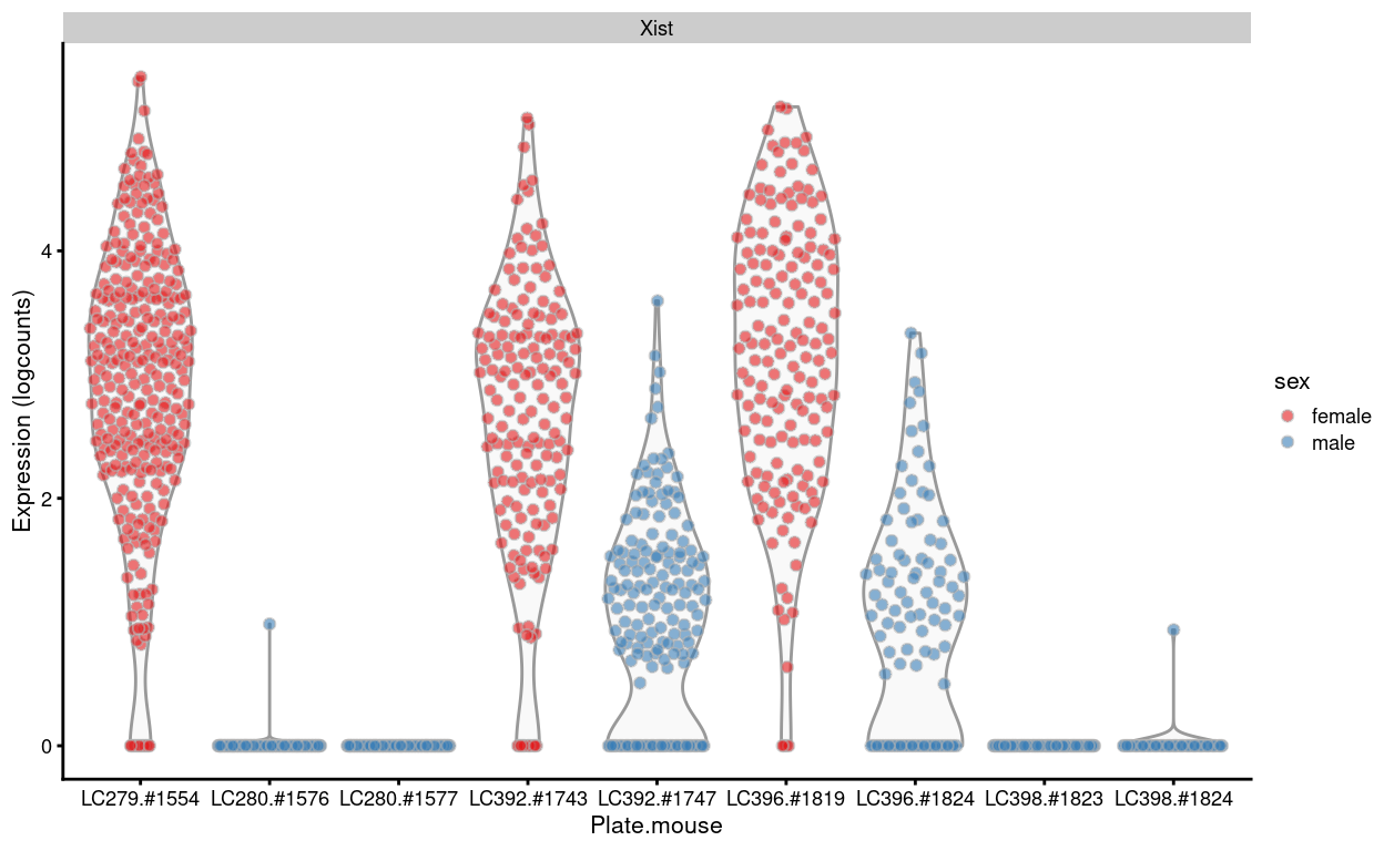
Figure 8: Expression of Xist in each sample.
Data integration
Motivation
Large single-cell RNA sequencing (scRNA-seq) projects usually need to generate data across multiple batches due to logistical constraints. However, the processing of different batches is often subject to uncontrollable differences, e.g., changes in operator, differences in reagent quality. This results in systematic differences in the observed expression in cells from different batches, which we refer to as “batch effects”. Batch effects are problematic as they can be major drivers of heterogeneity in the data, masking the relevant biological differences and complicating interpretation of the results.
Computational correction of these effects is critical for eliminating batch-to-batch variation, allowing data across multiple batches to be combined for common downstream analysis. However, existing methods based on linear models (Ritchie et al. 2015; Leek et al. 2012) assume that the composition of cell populations are either known or the same across batches. To overcome these limitations, bespoke methods have been developed for batch correction of single-cell data (Haghverdi et al. 2018; Butler et al. 2018; Lin et al. 2019) that do not require a priori knowledge about the composition of the population. This allows them to be used in workflows for exploratory analyses of scRNA-seq data where such knowledge is usually unavailable.
We will use the Mutual Nearest Neighbours (MNN) approach of Haghverdi et al. (2018), as implemented in the batchelor package, to perform data integration. The MNN approach does not rely on pre-defined or equal population compositions across batches, only requiring that a subset of the population be shared between batches.
Algorithm overview
Consider a cell \(a\) in batch \(A\), and identify the cells in batch \(B\) that are nearest neighbours to \(a\) in the expression space defined by the selected features (genes). Repeat this for a cell \(b\) in batch \(B\), identifying its nearest neighbours in
\(A\). Mutual nearest neighbours are pairs of cells from different batches that belong in each other’s set of nearest neighbours. The reasoning is that MNN pairs represent cells from the same biological state prior to the application of a batch effect6. Thus, the difference between cells in MNN pairs can be used as an estimate of the batch effect, the subtraction of which yields batch-corrected values.
Compared to linear regression, MNN correction does not assume that the population composition is the same or known beforehand. This is because it learns the shared population structure via identification of MNN pairs and uses this information to obtain an appropriate estimate of the batch effect. Instead, the key assumption of MNN-based approaches is that the batch effect is orthogonal to the biology in high-dimensional expression space. Violations reduce the effectiveness and accuracy of the correction, with the most common case arising from variations in the direction of the batch effect between clusters7.
Analysis
We treat each plate as a batch and let the MNN algorithm select the ‘best’ order for merging the plates.
One useful diagnostic of the MNN algorithm is the proportion of variance within each batch that is lost during MNN correction8. Large proportions of lost variance (>10%) suggest that correction is removing genuine biological heterogeneity. This would occur due to violations of the assumption of orthogonality between the batch effect and the biological subspace (Haghverdi et al. 2018). In this case, the proportion of lost variance is small, indicating that non-orthogonality is not a major concern.
| LC279 | LC280 | LC392 | LC396 | LC398 | |
|---|---|---|---|---|---|
| merge_1 | 0.0 | 2.3 | 2.4 | 0.0 | 0.0 |
| merge_2 | 0.0 | 2.2 | 1.9 | 3.3 | 0.0 |
| merge_3 | 5.7 | 1.2 | 1.0 | 0.9 | 0.0 |
| merge_4 | 0.7 | 0.6 | 0.6 | 0.6 | 2.6 |
Summary
The MNN algorithm returns two sets of corrected values for use in downstream analyses like clustering or visualization:
corrected: ‘Batch-corrected principal components’reconstructed: ‘Batch-corrected expression values’
The corrected data contains the low-dimensional corrected coordinates for all cells, which we will use in place of the PCs in our downstream analyses. The reconstructed data contains the corrected expression values for each gene in each cell, obtained by projecting the low-dimensional coordinates in corrected back into gene expression space. We do not recommend using the reconstructed data for anything other than visualization9.
Re-processing
We will use the MNN-corrected values in place of the PCs in our downstream analyses, such as UMAP and clustering10.
There are 7 clusters detected, shown on the UMAP plot Figure 9 and broken down by experimental factors in Figure 10.
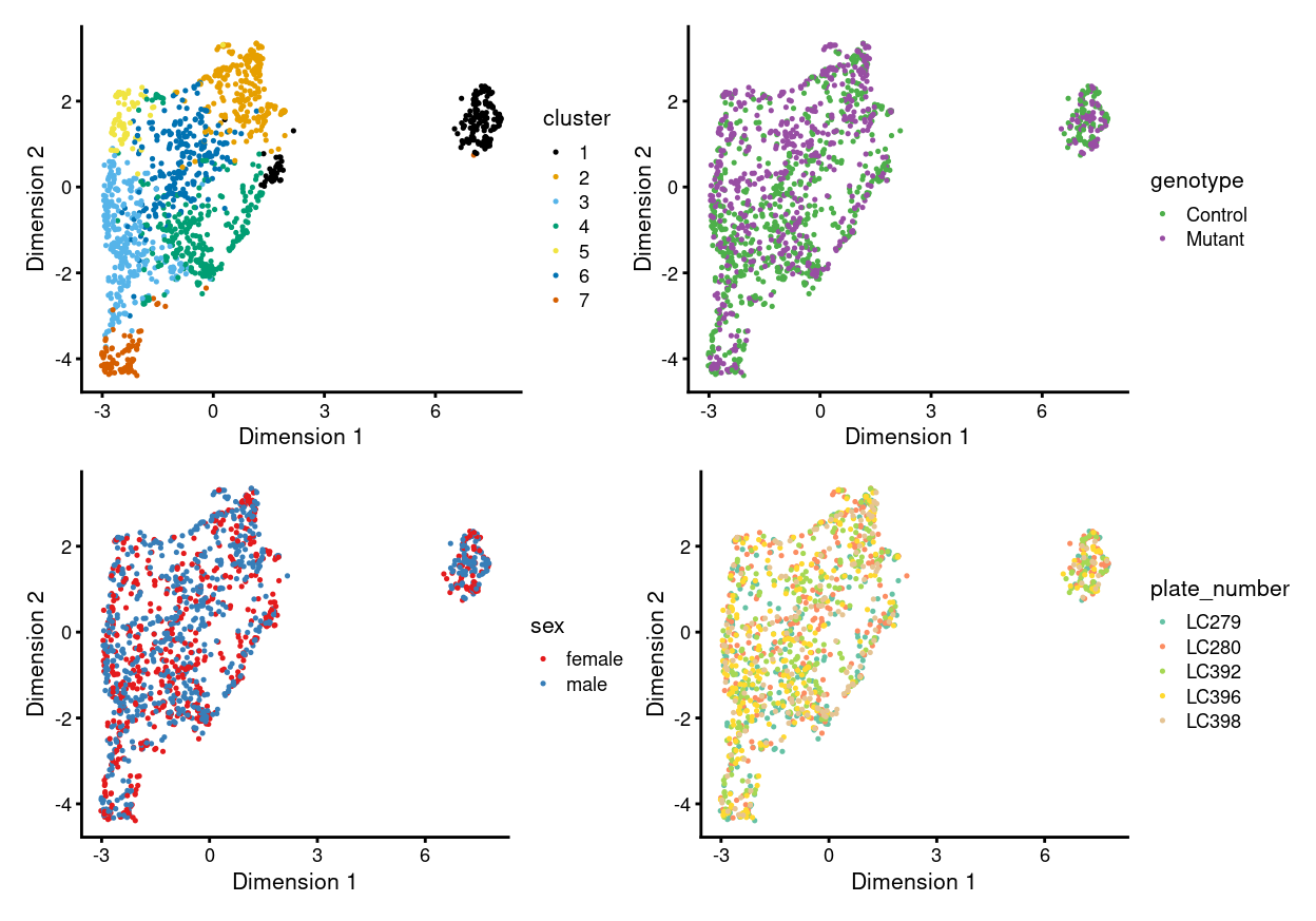
Figure 9: UMAP plot, where each point represents a cell and is coloured according to the legend.
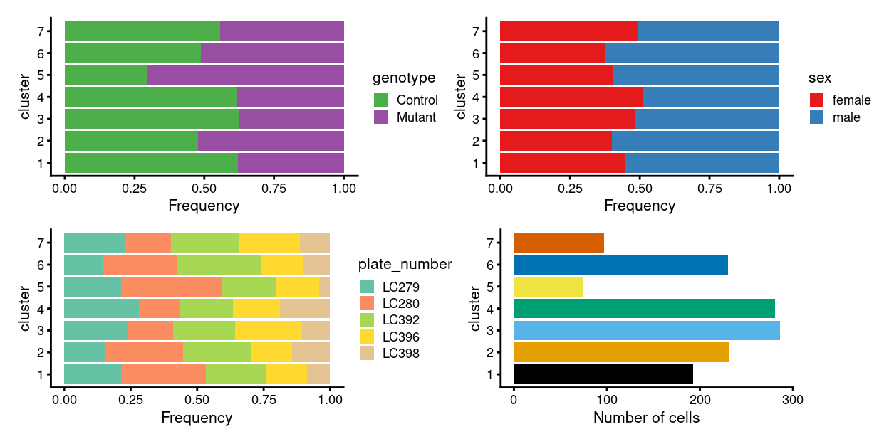
Figure 10: Breakdown of clusters by experimental factors.
Notably:
- Now, none of the clusters are highly plate-specific.
- Now, there are clusters that are somewhat genotype-specific.
Concluding remarks
The processed SingleCellExperiment object is available (see data/SCEs/C075_Grant_Coultas.cells_selected.SCE.rds). This will be used in downstream analyses, e.g., identifying cluster marker genes and refining the cell labels.
Additional information
The following are available on request:
- Full CSV tables of any data presented.
- PDF/PNG files of any static plots.
Session info
─ Session info ─────────────────────────────────────────────────────
 setting  value
 version  R version 4.0.0 (2020-04-24)
 os       CentOS Linux 7 (Core)
 system   x86_64, linux-gnu
 ui       X11
 language (EN)
 collate  en_US.UTF-8
 ctype    en_US.UTF-8
 tz       Australia/Melbourne
 date     2020-10-01

─ Packages ─────────────────────────────────────────────────────────
 ! package              * version  date       lib source
 P assertthat             0.2.1    2019-03-21 [?] CRAN (R 4.0.0)
 P backports              1.1.8    2020-06-17 [?] CRAN (R 4.0.0)
 P batchelor            * 1.4.0    2020-04-27 [?] Bioconductor
 P beeswarm               0.2.3    2016-04-25 [?] CRAN (R 4.0.0)
 P Biobase              * 2.48.0   2020-04-27 [?] Bioconductor
 P BiocGenerics         * 0.34.0   2020-04-27 [?] Bioconductor
 P BiocManager            1.30.10  2019-11-16 [?] CRAN (R 4.0.0)
 P BiocNeighbors          1.6.0    2020-04-27 [?] Bioconductor
 P BiocParallel         * 1.22.0   2020-04-27 [?] Bioconductor
 P BiocSingular           1.4.0    2020-04-27 [?] Bioconductor
 P BiocStyle              2.16.0   2020-04-27 [?] Bioconductor
 P bitops                 1.0-6    2013-08-17 [?] CRAN (R 4.0.0)
 P cellranger             1.1.0    2016-07-27 [?] CRAN (R 4.0.0)
 P cli                    2.0.2    2020-02-28 [?] CRAN (R 4.0.0)
 P colorspace             1.4-1    2019-03-18 [?] CRAN (R 4.0.0)
 P cowplot              * 1.0.0    2019-07-11 [?] CRAN (R 4.0.0)
 P crayon                 1.3.4    2017-09-16 [?] CRAN (R 4.0.0)
 P crosstalk              1.1.0.1  2020-03-13 [?] CRAN (R 4.0.0)
 P DelayedArray         * 0.14.1   2020-07-14 [?] Bioconductor
 P DelayedMatrixStats     1.10.1   2020-07-03 [?] Bioconductor
 P digest                 0.6.25   2020-02-23 [?] CRAN (R 4.0.0)
 P distill                0.8      2020-06-04 [?] CRAN (R 4.0.0)
 P dplyr                  1.0.0    2020-05-29 [?] CRAN (R 4.0.0)
 P dqrng                  0.2.1    2019-05-17 [?] CRAN (R 4.0.0)
 P DT                     0.14     2020-06-24 [?] CRAN (R 4.0.0)
 P edgeR                * 3.30.3   2020-06-02 [?] Bioconductor
 P ellipsis               0.3.1    2020-05-15 [?] CRAN (R 4.0.0)
 P evaluate               0.14     2019-05-28 [?] CRAN (R 4.0.0)
 P fansi                  0.4.1    2020-01-08 [?] CRAN (R 4.0.0)
 P farver                 2.0.3    2020-01-16 [?] CRAN (R 4.0.0)
 P FNN                    1.1.3    2019-02-15 [?] CRAN (R 4.0.0)
 P generics               0.0.2    2018-11-29 [?] CRAN (R 4.0.0)
 P GenomeInfoDb         * 1.24.2   2020-06-15 [?] Bioconductor
 P GenomeInfoDbData       1.2.3    2020-05-18 [?] Bioconductor
 P GenomicRanges        * 1.40.0   2020-04-27 [?] Bioconductor
 P ggbeeswarm             0.6.0    2017-08-07 [?] CRAN (R 4.0.0)
 P ggplot2              * 3.3.2    2020-06-19 [?] CRAN (R 4.0.0)
 P Glimma               * 1.16.0   2020-04-27 [?] Bioconductor
 P glue                   1.4.1    2020-05-13 [?] CRAN (R 4.0.0)
 P gridExtra              2.3      2017-09-09 [?] CRAN (R 4.0.0)
 P gtable                 0.3.0    2019-03-25 [?] CRAN (R 4.0.0)
 P here                 * 0.1      2017-05-28 [?] CRAN (R 4.0.0)
 P highr                  0.8      2019-03-20 [?] CRAN (R 4.0.0)
 P htmltools              0.5.0    2020-06-16 [?] CRAN (R 4.0.0)
 P htmlwidgets            1.5.1    2019-10-08 [?] CRAN (R 4.0.0)
 P igraph                 1.2.5    2020-03-19 [?] CRAN (R 4.0.0)
 P IRanges              * 2.22.2   2020-05-21 [?] Bioconductor
 P irlba                  2.3.3    2019-02-05 [?] CRAN (R 4.0.0)
 P jsonlite               1.7.0    2020-06-25 [?] CRAN (R 4.0.0)
 P knitr                  1.29     2020-06-23 [?] CRAN (R 4.0.0)
 P labeling               0.3      2014-08-23 [?] CRAN (R 4.0.0)
 P lattice                0.20-41  2020-04-02 [?] CRAN (R 4.0.0)
 P lifecycle              0.2.0    2020-03-06 [?] CRAN (R 4.0.0)
 P limma                * 3.44.3   2020-06-12 [?] Bioconductor
 P locfit                 1.5-9.4  2020-03-25 [?] CRAN (R 4.0.0)
 P magrittr               1.5      2014-11-22 [?] CRAN (R 4.0.0)
 P Matrix                 1.2-18   2019-11-27 [?] CRAN (R 4.0.0)
 P matrixStats          * 0.56.0   2020-03-13 [?] CRAN (R 4.0.0)
 P msigdbr              * 7.1.1    2020-05-14 [?] CRAN (R 4.0.0)
 P munsell                0.5.0    2018-06-12 [?] CRAN (R 4.0.0)
 P patchwork            * 1.0.1    2020-06-22 [?] CRAN (R 4.0.0)
 P pheatmap             * 1.0.12   2019-01-04 [?] CRAN (R 4.0.0)
 P pillar                 1.4.6    2020-07-10 [?] CRAN (R 4.0.0)
 P pkgconfig              2.0.3    2019-09-22 [?] CRAN (R 4.0.0)
 P Polychrome             1.2.5    2020-03-29 [?] CRAN (R 4.0.0)
 P purrr                  0.3.4    2020-04-17 [?] CRAN (R 4.0.0)
 P R6                     2.4.1    2019-11-12 [?] CRAN (R 4.0.0)
 P RColorBrewer           1.1-2    2014-12-07 [?] CRAN (R 4.0.0)
 P Rcpp                   1.0.5    2020-07-06 [?] CRAN (R 4.0.0)
 P RCurl                  1.98-1.2 2020-04-18 [?] CRAN (R 4.0.0)
 P readxl                 1.3.1    2019-03-13 [?] CRAN (R 4.0.0)
 P rlang                  0.4.7    2020-07-09 [?] CRAN (R 4.0.0)
 P rmarkdown              2.3      2020-06-18 [?] CRAN (R 4.0.0)
 P rprojroot              1.3-2    2018-01-03 [?] CRAN (R 4.0.0)
 P RSpectra               0.16-0   2019-12-01 [?] CRAN (R 4.0.0)
 P rsvd                   1.0.3    2020-02-17 [?] CRAN (R 4.0.0)
 P S4Vectors            * 0.26.1   2020-05-16 [?] Bioconductor
 P scales                 1.1.1    2020-05-11 [?] CRAN (R 4.0.0)
 P scater               * 1.16.2   2020-06-26 [?] Bioconductor
 P scatterplot3d          0.3-41   2018-03-14 [?] CRAN (R 4.0.0)
 P scran                * 1.16.0   2020-04-27 [?] Bioconductor
 P sessioninfo            1.1.1    2018-11-05 [?] CRAN (R 4.0.0)
 P SingleCellExperiment * 1.10.1   2020-04-28 [?] Bioconductor
 P statmod                1.4.34   2020-02-17 [?] CRAN (R 4.0.0)
 P stringi                1.4.6    2020-02-17 [?] CRAN (R 4.0.0)
 P stringr                1.4.0    2019-02-10 [?] CRAN (R 4.0.0)
 P SummarizedExperiment * 1.18.2   2020-07-09 [?] Bioconductor
 P tibble                 3.0.3    2020-07-10 [?] CRAN (R 4.0.0)
 P tidyr                  1.1.0    2020-05-20 [?] CRAN (R 4.0.0)
 P tidyselect             1.1.0    2020-05-11 [?] CRAN (R 4.0.0)
 P uwot                   0.1.8    2020-03-16 [?] CRAN (R 4.0.0)
 P vctrs                  0.3.2    2020-07-15 [?] CRAN (R 4.0.0)
 P vipor                  0.4.5    2017-03-22 [?] CRAN (R 4.0.0)
 P viridis                0.5.1    2018-03-29 [?] CRAN (R 4.0.0)
 P viridisLite            0.3.0    2018-02-01 [?] CRAN (R 4.0.0)
 P withr                  2.2.0    2020-04-20 [?] CRAN (R 4.0.0)
 P xfun                   0.15     2020-06-21 [?] CRAN (R 4.0.0)
 P XVector                0.28.0   2020-04-27 [?] Bioconductor
 P yaml                   2.2.1    2020-02-01 [?] CRAN (R 4.0.0)
 P zlibbioc               1.34.0   2020-04-27 [?] Bioconductor

[1] /stornext/General/data/user_managed/grpu_mritchie_1/hickey/SCORE/C075_Grant_Coultas/renv/library/R-4.0/x86_64-pc-linux-gnu
[2] /tmp/RtmpImljK7/renv-system-library
[3] /stornext/System/data/apps/R/R-4.0.0/lib64/R/library

 P ── Loaded and on-disk path mismatch.
Butler, A., P. Hoffman, P. Smibert, E. Papalexi, and R. Satija. 2018. “Integrating Single-Cell Transcriptomic Data Across Different Conditions, Technologies, and Species.” Nat. Biotechnol. 36 (5): 411–20.
Haghverdi, L., A. T. L. Lun, M. D. Morgan, and J. C. Marioni. 2018. “Batch Effects in Single-Cell Rna-Sequencing Data Are Corrected by Matching Mutual Nearest Neighbors.” Nat. Biotechnol., April.
Leek, J. T., W. E. Johnson, H. S. Parker, A. E. Jaffe, and J. D. Storey. 2012. “The Sva Package for Removing Batch Effects and Other Unwanted Variation in High-Throughput Experiments.” Bioinformatics 28 (6): 882–83.
Lin, Y., S. Ghazanfar, K. Y. X. Wang, J. A. Gagnon-Bartsch, K. K. Lo, X. Su, Z. G. Han, et al. 2019. “ScMerge Leverages Factor Analysis, Stable Expression, and Pseudoreplication to Merge Multiple Single-Cell Rna-Seq Datasets.” Proc. Natl. Acad. Sci. U.S.A. 116 (20): 9775–84.
Ritchie, M. E., B. Phipson, D. Wu, Y. Hu, C. W. Law, W. Shi, and G. K. Smyth. 2015. “Limma Powers Differential Expression Analyses for Rna-Sequencing and Microarray Studies.” Nucleic Acids Res. 43 (7): e47.
Xu, C., and Z. Su. 2015. “Identification of Cell Types from Single-Cell Transcriptomes Using a Novel Clustering Method.” Bioinformatics 31 (12): 1974–80.
But see the ‘Data integration’ section of this report for an exception to the rule.↩︎
Email 2020-05-06.↩︎
Effect sizes for each comparison are reported as log2-fold changes in the proportion of expressing cells in one group over the proportion in another group.↩︎
Meeting between Daniela, Zoe and I on 2020-03-06 and in email on 2020-07-19.↩︎
Mouse
#1824acts as a control sample on two plates.↩︎Nonetheless, the assumption is usually reasonable as a random vector is very likely to be orthogonal in high-dimensional space.↩︎
Specifically, this refers to the within-batch variance that is removed during orthogonalization with respect to the average correction vector at each merge step.↩︎
See here for a detailed explanation of this recommendation.↩︎
At this point, it is also tempting to use the corrected expression values for gene-based analyses like DE-based marker gene detection. This is not generally recommended as an arbitrary correction algorithm is not obliged to preserve the magnitude (or even direction) of differences in per-gene expression when attempting to align multiple batches.↩︎