Table of Contents
Motivation
A powerful use of scRNA-seq technology lies in the design of replicated multi-condition experiments to detect changes in composition or expression between conditions. For example, a researcher could use this strategy to detect changes in cell type abundance after drug treatment (Richard et al. 2018) or genetic modifications (Scialdone et al. 2016). This provides more biological insight than conventional scRNA-seq experiments involving only one biological condition, especially if we can relate population changes to specific experimental perturbations.
Differential analyses of multi-condition scRNA-seq experiments can be broadly split into two categories - differential expression (DE) and differential abundance (DA) analyses. The former tests for changes in expression between conditions for cells of the same type that are present in both conditions, while the latter tests for changes in the composition of cell types (or states, etc.) between conditions.
For this experiment, we are interested in identifying differences between genotype. We are not interested in the differences due to plate_number, sex, and mouse, so we will block on these variables where possible.
Setting up the data
We start from the preprocessed SingleCellExperiment object created in ‘Annotating the Grant (C075) retinal epithelial cells data set’.
As a reminder, Zoe requested that clusters 3, 4, and 6 be aggregated to create cell labels for the purposes of differential analyses. Figure 1 shows the cluster labels and the cell labels (i.e. Zoe’s aggregated cluster labels) on the UMAP plot.
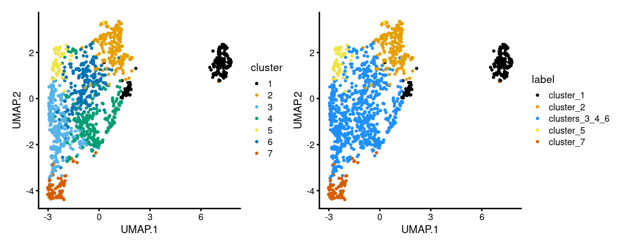
Figure 1: UMAP plot, where each point represents a cell and is coloured according to the legend.
Figure 2 breaks down the cell labels by key experimental factors.
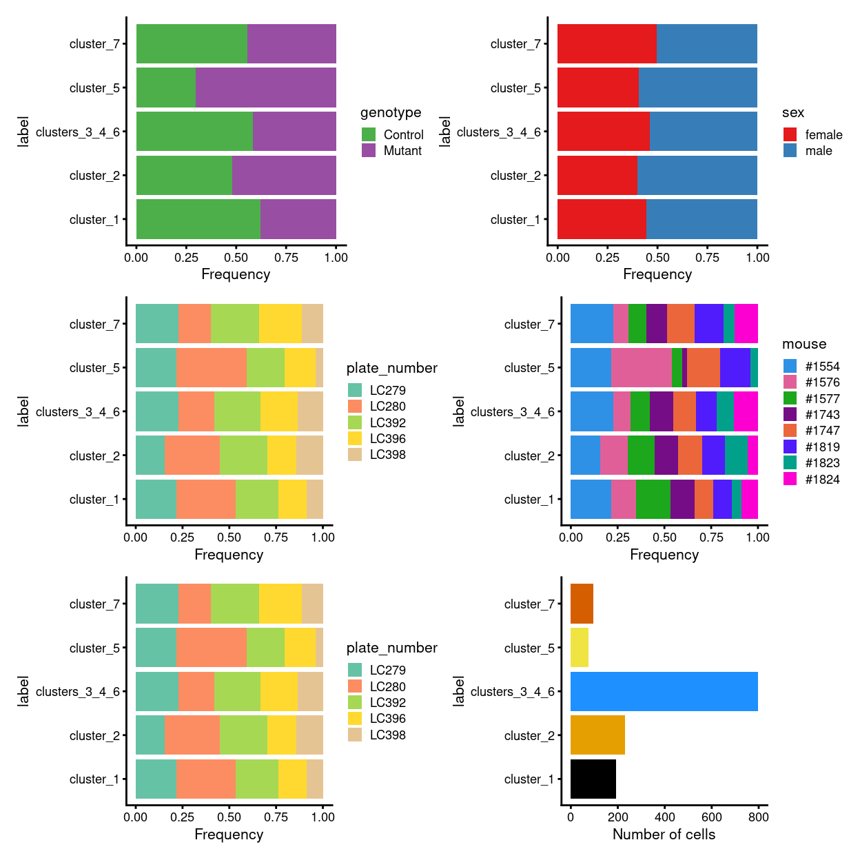
Figure 2: Breakdown of cell labels by experimental factors.
Figure 3 is a reminder that the mice are partially matched by genotype (and sibship) within each plate.
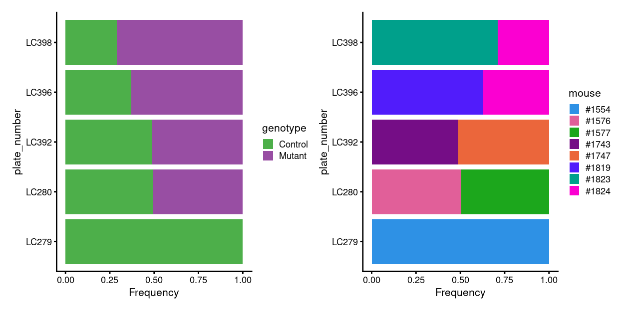
Figure 3: Breakdown of plates by experimental factors.
Differential abundance between conditions
Overview
In a DA analysis, we test for significant changes in per-label cell abundance across conditions. This will reveal which cell types are depleted or enriched with differences in genotype, which is arguably just as interesting as changes in expression within each cell type. The DA analysis has a long history in flow cytometry (Finak et al. 2015; Lun, Richard, and Marioni 2017) where it is routinely used to examine the effects of different conditions on the composition of complex cell populations. By performing it here, we effectively treat scRNA-seq as a “super-FACS” technology for defining relevant subpopulations using the entire transcriptome.
We prepare for the DA analysis by quantifying the number of cells assigned to each label. The table below and Figure 4 summarise the number of cells assigned to each label per plate. In this case, we are aiming to identify labels that change in abundance among the Mutant cells compared to the Control cells. Visually, cluster_5 has a strong and consistent change in abundance between genotypes.
| genotype | sample | cluster_1 | cluster_2 | clusters_3_4_6 | cluster_5 | cluster_7 |
|---|---|---|---|---|---|---|
| Control | LC279.#1554 | 42 | 36 | 181 | 16 | 22 |
| Control | LC280.#1577 | 36 | 33 | 81 | 4 | 9 |
| Control | LC392.#1743 | 25 | 29 | 99 | 2 | 11 |
| Control | LC396.#1824 | 10 | 8 | 71 | 0 | 7 |
| Control | LC398.#1824 | 7 | 5 | 32 | 0 | 5 |
| Mutant | LC280.#1576 | 25 | 35 | 74 | 24 | 8 |
| Mutant | LC392.#1747 | 19 | 30 | 97 | 13 | 14 |
| Mutant | LC396.#1819 | 19 | 28 | 88 | 12 | 15 |
| Mutant | LC398.#1823 | 10 | 28 | 74 | 3 | 6 |
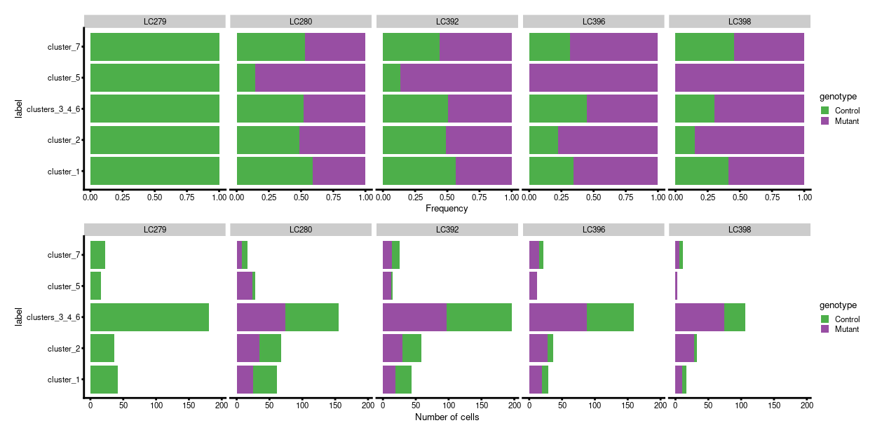
Figure 4: Breakdown of labels by experimental factors.
Performing the DA anlaysis
Overview
Our DA analysis will be performed with the edgeR package. This allows us to take advantage of the negative binomial generalized linear model (NB GLM) methods to model overdispersed count data in the presence of limited replication - except that the counts are not of reads per gene, but of cells per label (Lun, Richard, and Marioni 2017). The aim is to share information across labels to improve our estimates of the biological variability in cell abundance between replicates.
Statistical methodology
Pre-processing
We filter out low-abundance labels to avoid cluttering the result table with very rare subpopulations that contain only a handful of cells.
For a DA analysis of cluster abundances, filtering is generally not required as most clusters will not be of low-abundance (otherwise there would not have been enough evidence to define the cluster in the first place), but in this case we filter out .
Statistical methodology
Unlike a differential expression analyses, we do not perform an additional normalization step. This means that we are only normalizing based on the “library size”, i.e., the total number of cells in each sample. Any changes we detect between conditions will subsequently represent differences in the proportion of cells in each cluster. The motivation behind this decision is discussed in more detail in Handling composition effects.
We set up the design matrix to block on the sample-to-sample differences across different mice and plates, while retaining an additive term that represents the effect of genotype. Here, the log-fold change in our model refers to the change in cell abundance associated with genotype, rather than the change in gene expression.
We estimate the NB dispersion and QL dispersion for each label1.
Analysis using cell labels
We test for differences in abundance between Mutant and Control samples using glmQLFTest() function from the edgeR package to obtain a list of genotype-associated labels.
We find one label, cluster_5, is strongly associated with genotype at a false discovery rate of 5%, as shown in the table below.
| logFC | logCPM | F | PValue | FDR | |
|---|---|---|---|---|---|
| cluster_5 | 2.8226956 | 15.97425 | 42.6920499 | 0.0000095 | 0.0000473 |
| cluster_1 | -0.4109530 | 17.17182 | 3.6967730 | 0.0819777 | 0.1518905 |
| clusters_3_4_6 | -0.1999776 | 19.12147 | 3.4711672 | 0.0911343 | 0.1518905 |
| cluster_2 | 0.3268769 | 17.41668 | 2.9012653 | 0.1237290 | 0.1546612 |
| cluster_7 | 0.0015624 | 16.29626 | 0.0000263 | 0.9960360 | 0.9960360 |
Handling composition effects
Our default approach for normalization in a differential abundance analysis is to only normalize based on the total number of cells in each sample, which means that we are effectively testing for differential proportions between conditions.
Unfortunately, the use of the total number of cells leaves us susceptible to composition effects. For example, a large increase in abundance for one cell subpopulation will introduce decreases in proportion for all other subpopulations - which is technically correct, but may be misleading if one concludes that those other subpopulations are decreasing in abundance of their own volition. If composition biases are proving problematic for interpretation of DA results, we have several avenues for removing them or mitigating their impact.
Differential expression between conditions
Creating pseudo-bulk samples
The most obvious differential analysis is to look for changes in expression between conditions. We perform the DE analysis separately for each label to identify cell type-specific transcriptional effects of genotype. The actual DE testing is performed on “pseudo-bulk” expression profiles (Tung et al. 2017), generated by summing counts together for all cells with the same combination of label and sample. This leverages the resolution offered by single-cell technologies to define the labels, and combines it with the statistical rigor of existing methods for DE analyses involving a small number of samples.
At this point, it is worth reflecting on the motivations behind the use of pseudo-bulking:
- Larger counts are more amenable to standard DE analysis pipelines designed for bulk RNA-seq data. Normalization is more straightforward and certain statistical approximations are more accurate2.
- Collapsing cells into samples reflects the fact that our biological replication occurs at the sample level (A. T. Lun and Marioni 2017). Each sample is represented no more than once for each condition, avoiding problems from unmodelled correlations between samples. Supplying the per-cell counts directly to a DE analysis pipeline would imply that each cell is an independent biological replicate, which is not true from an experimental perspective3.
- Variance between cells within each sample is masked, provided it does not affect variance across (replicate) samples. This avoids penalizing DEGs that are not uniformly up- or down-regulated for all cells in all samples of one condition. Masking is generally desirable as DEGs - unlike marker genes - do not need to have low within-sample variance to be interesting, e.g., if the treatment effect is consistent across replicate populations but heterogeneous on a per-cell basis4.
Performing the DE analysis
Overview
The DE analysis will be performed using quasi-likelihood (QL) methods from the edgeR package (Robinson, McCarthy, and Smyth 2010; Chen, Lun, and Smyth 2014). This uses a negative binomial generalized linear model (NB GLM) to handle overdispersed count data in experiments with limited replication. In our case, we have biological variation with four replicates per condition, with the replicates for each condition partially paired as genotype-discordant siblings within each plate, so edgeR (or its contemporaries) is a natural choice for the analysis.
We do not use all labels for GLM fitting as the strong DE between labels makes it difficult to compute a sensible average abundance to model the mean-dispersion trend. Moreover, label-specific batch effects would not be easily handled with a single additive term in the design matrix for the batch.
Statistical methodology and considerations
Pre-processing
A typical step in bulk RNA-seq data analyses is to remove samples with very low library sizes due to failed library preparation or sequencing. The very low counts in these samples can be troublesome in downstream steps such as normalization or for some statistical approximations used in the DE analysis. In our situation, this is equivalent to removing label-sample combinations that have very few or lowly-sequenced cells. The exact definition of “very low” will vary, but in this case we remove combinations containing fewer than 2 cells. This is much lower than generally recommended5 but here we are limited by the small numbers of cells/sample that were processed.
Another typical step in bulk RNA-seq analyses is to remove genes that are lowly expressed. This reduces computational work, improves the accuracy of mean-variance trend modelling and decreases the severity of the multiple testing correction. Genes are discarded if they are not expressed above a log-CPM threshold in a minimum number of samples (determined from the size of the smallest treatment group in the experimental design).
Finally, we correct for composition biases by computing normalization factors with the trimmed mean of M-values method (Robinson and Oshlack 2010). We do not need the bespoke single-cell methods used earlier in this analysis, as the counts for our pseudo-bulk samples are large enough to apply bulk normalization methods.
Statistical modelling
We set up the design matrix to block on the sample-to-sample differences across different mice and plates, while retaining an additive term that represents the effect of genotype. The latter is represented in our model as the log-fold change in gene expression in Mutant cells over their Control counterparts within the same label. Our aim is to test whether this log-fold change is significantly different from zero.
We estimate the negative binomial (NB) dispersions to model the mean-variance trend, which is not easily accommodated by QL dispersions alone due to the quadratic nature of the NB mean-variance trend. We also estimate the quasi-likelihood dispersions to model the uncertainty and variability of the per-gene variance, which is not well handled by the NB dispersions. So the two dispersion types complement each other in the final analysis.
We test for differences in expression due to genotype. DEGs are defined as those with non-zero log-fold changes at a false discovery rate of 5%.
Analysis using cell labels
As noted in Setting up the data, we start by using the aggregated cluster labels as the cell labels.
Now that we have laid out the theory underlying the DE analysis, we repeat this process for each of the labels to identify genotype-associated DE in each cell type. To prepare for this, we filter out all sample-label combinations with insufficient cells.
We then apply the pseudoBulkDGE() function from the scran package to obtain a list of genotype-associated DE genes for each label. This function puts some additional effort into automatically dealing with labels that are not represented in both Mutant and Control cells, for which a DE analysis between conditions is meaningless or are not represented in a sufficient number of replicate samples to enable modelling of biological variability.
Figure 5 summarises the DEGs using a heatmap of pseudobulk-level log-expression values. In general, there seems to be little differential expression that is associated with genotype, except within clusters_3_4_6.
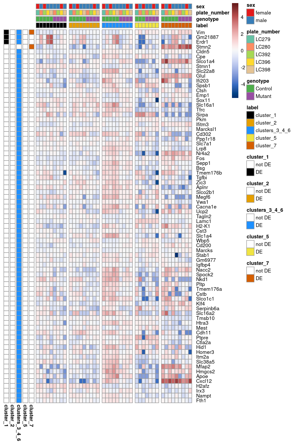
Figure 5: Heatmap of pseudobulk-level log-expression values normalized to the mean of all samples in the filtered data; rows correspond to genes, columns to label-sample combinations. Included is the union of DEGs detected (FDR < r fdr) across all labels. Data is split horizontally by label and rows are annotated to show in which label(s) each gene is DE.
The following table gives the number of DEGs at a FDR of 5% for each label.
| -1 | 0 | 1 | NA | |
|---|---|---|---|---|
| cluster_1 | 2 | 6698 | 1 | 26954 |
| cluster_2 | 0 | 7806 | 0 | 25849 |
| cluster_5 | 0 | 4399 | 0 | 29256 |
| cluster_7 | 0 | 1521 | 2 | 32132 |
| clusters_3_4_6 | 56 | 9453 | 20 | 24126 |
Note that genes listed as NA in the above table were either filtered out as low-abundance genes for a given label’s analysis, or the comparison of interest was not possible for a particular label, e.g., due to lack of residual degrees of freedom or an absence of samples from both conditions. If it is necessary to extract statistics in the absence of replicates, several strategies can be applied such as reducing the complexity of the model or using a predefined value for the NB dispersion.
Please see output/DEGs/ for spreadsheets of these DEG lists, including results of GO and KEGG analyses using the goana() and kegga() functions from the limma package6, and output/glimma-plots for interactive Glimma plots of the differential expression results. The Glimma plots show the pseudobulk data for that label on the left-hand side and the single-cell data for that label on the right-hand side. The single-cell data are plotted per sample using abbreviated sample labels, e.g., C.LC280 means “control mouse on plate LC280”, M.LC280 means “mutate mouse on plate LC280”, etc.
Analysis using ‘coarser’ labels
As noted in Pre-processing, by only requiring 2 cells/label/mouse we are using fewer cells/label/sample than the generally recommended minimum of 100. If we had more cells/label/sample then we would expect to increase our true positive rate, i.e. we would have greater statistical power to identify DEGs (Crowell et al. 2019). Fortunately, Crowell et al. (2019) also found that the false discovery rate is not greatly affected by the choice of minimum number of cells, so we are probably not at risk of making more false discoveries by using a low minimum number of cells/label/sample.
To increase the number of cells/label/sample would require one or more of:
- The acquisition of additional cells (i.e. more experiments)
- The use of ‘coarser’ labels (i.e. aggregation of the existing labels)
- The use of ‘coarser’ samples (i.e. aggregation of the existing samples)
The first is probably not feasible while the latter ignores the known biological (e.g., mouse) and technical (e.g., plate) variability between replicates samples. We are therefore left with using ‘coarser’ labels.
To generate ‘coarser’ labels, we can simply ignore the clustering results entirely (i.e. the label is ignoring_clusters). In doing so we are implicitly accepting that any DEGs identified in the subsequent analysis are at increased chance of reflecting differences in ‘cell type’ between genotypes (i.e. differential abundance) rather than differential gene expression between genotypes per se.
Figure 6 summarises the DEGs using a heatmap of pseudobulk-level log-expression values. There are more DEGs detected when we use the ‘coarser’ labels.
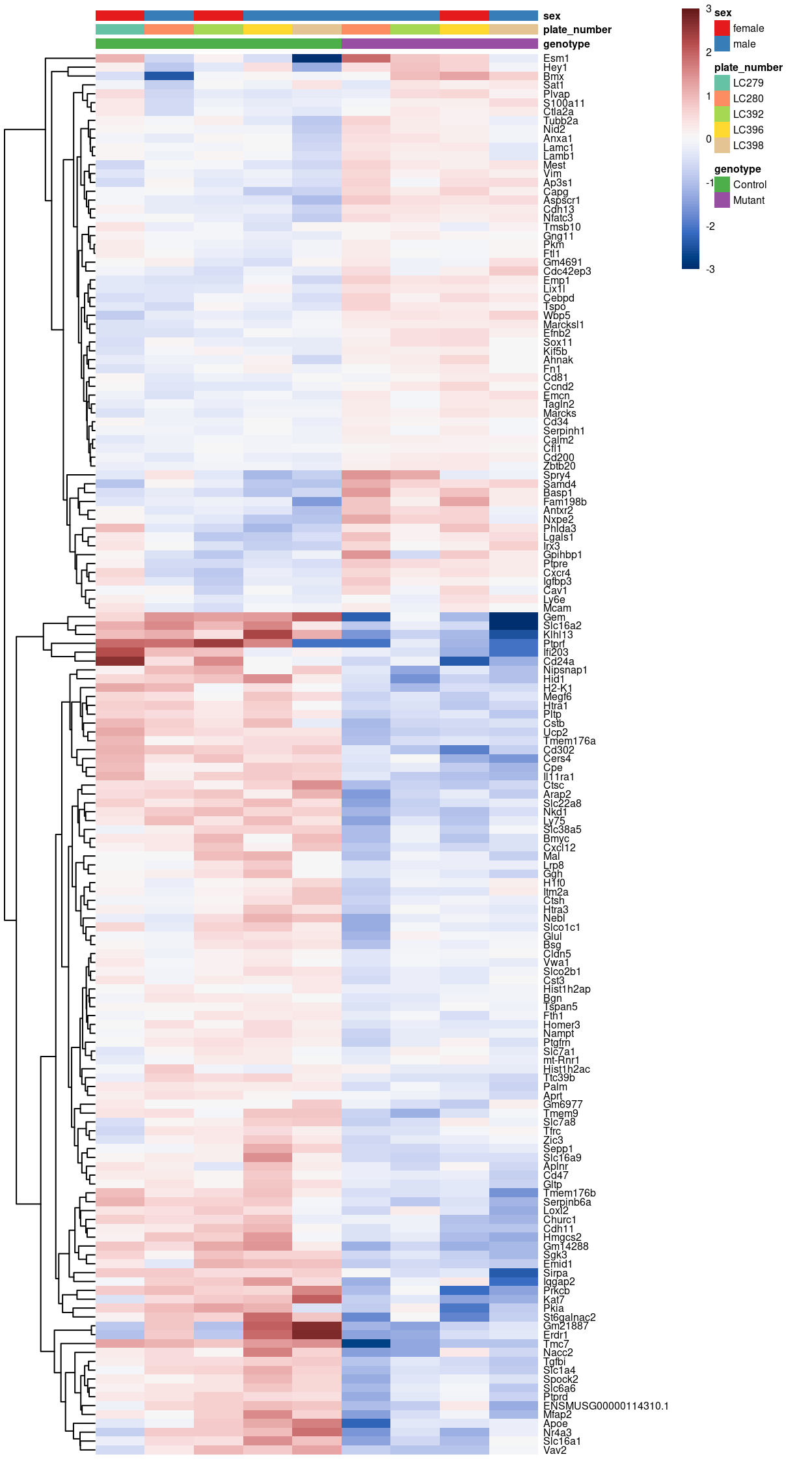
Figure 6: Heatmap of pseudobulk-level log-expression values normalized to the mean of all samples in the filtered data; rows correspond to genes, columns to label-sample combinations. Included is the union of DEGs detected (FDR < r fdr).
The following table gives the number of DEGs at a FDR of 5%.
| -1 | 0 | 1 | NA | |
|---|---|---|---|---|
| ignoring_clusters | 95 | 12171 | 63 | 21326 |
Please see output/DEGs/ for spreadsheets of these DEG lists, including results of GO and KEGG analyses using the goana() and kegga() functions from the limma package7, and output/glimma-plots for interactive Glimma plots of the differential expression results. The Glimma plots show the pseudobulk data for that label on the left-hand side and the single-cell data for that label on the right-hand side. The single-cell data are plotted per sample using abbreviated sample labels, e.g., C.LC280 means “control mouse on plate LC280”, M.LC280 means “mutant mouse on plate LC280”, etc.
Futher gene set testing
As noted above, the GO and KEGG results computed so far have been non-directional (i.e. they don’t incorporate the direction of the log-fold change). With a bit more work we can incorporate the log-fold change to create more specific GO and KEGG analyses. Please see the CSV files with “directional” in the file name in output/DEGs/ for spreadsheets of directional GO and KEGG results8.
In addition to the GO and KEGG analyses, we perform ‘rotation gene set tests’ using the fry() function in the edgeR (Wu et al. 2010). This tests whether a set of genes is DE, assessing the set of genes as a whole. Gene set tests consider all the genes in the specified set and do not depend on any pre-emptive significance cut off. The set of genes can be chosen to be representative of any pathway or phenotype of interest. Zoe sent me such a set of genes (see data/zoes_marker_genes/20200728 barcode plot gene lists.xlsx).
The results of the fry() analysis are shown below.
| Gene set | NGenes | Direction | PValue | FDR | PValue.Mixed | FDR.Mixed |
|---|---|---|---|---|---|---|
| Notch signaling pathway | 41 | Up | 0.1349801 | 0.5324207 | 0.0003475 | 0.0005792 |
| Vegf signaling pathway | 39 | Down | 0.2541349 | 0.5324207 | 0.0000913 | 0.0002282 |
| Hif1 signaling pathway | 78 | Down | 0.3194524 | 0.5324207 | 0.0008983 | 0.0011229 |
| FoxO signaling pathway | 92 | Up | 0.7723357 | 0.8357779 | 0.0000386 | 0.0001932 |
| TGF-beta signaling pathway | 49 | Down | 0.8357779 | 0.8357779 | 0.0670270 | 0.0670270 |
Figure 7 visualises the enrichment of the each gene set using a barcode enrichment plot.
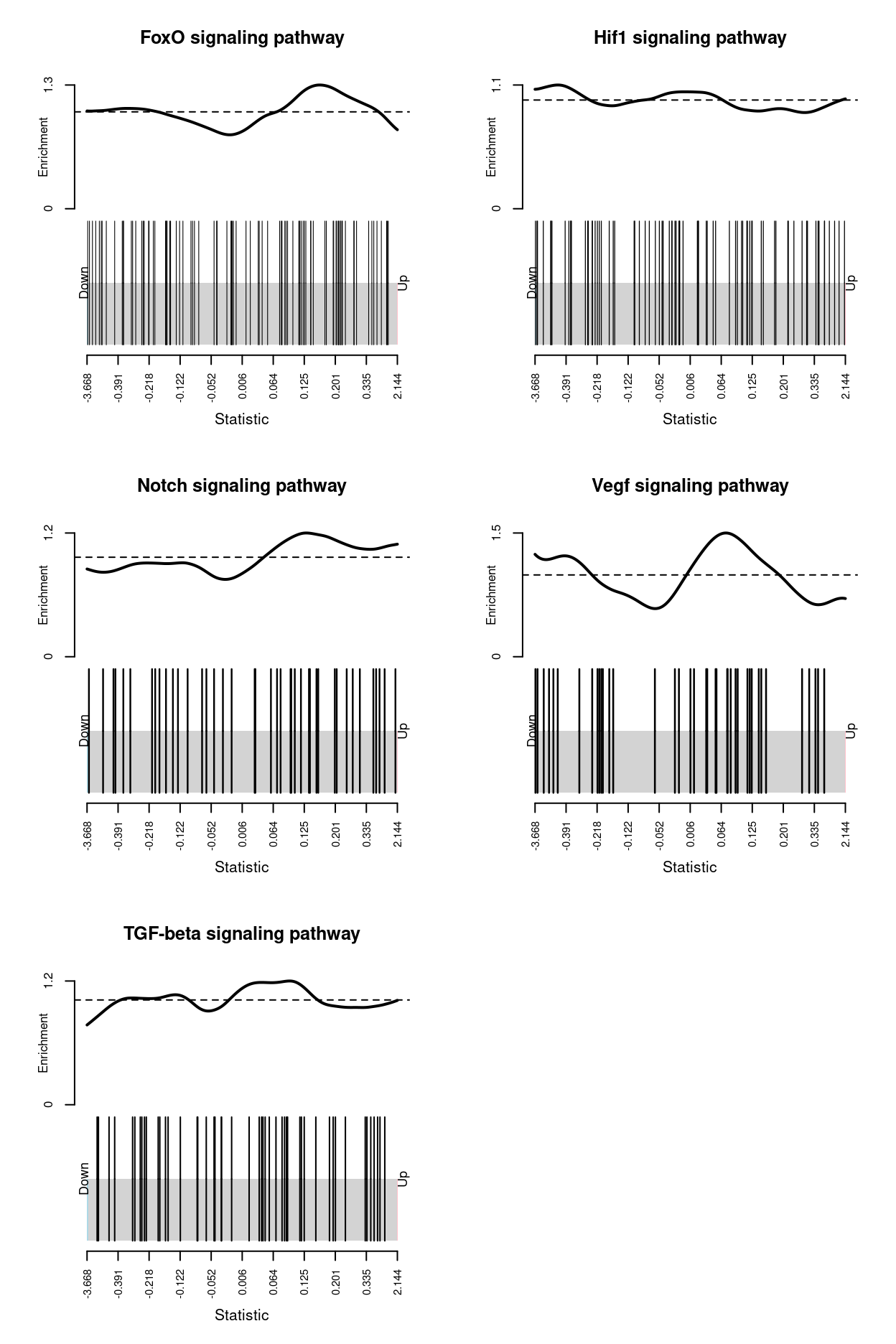
Figure 7: Barcode plot of the gene set supplied by Zoe. An enrichment line shows the relative enrichment of the vertical bars in each part of the plot is displayed.
Finally, Figure 8 visualises the enrichment of the ignoring_clusters DEGs amongst the within-label DE results using barcode enrichment plots.
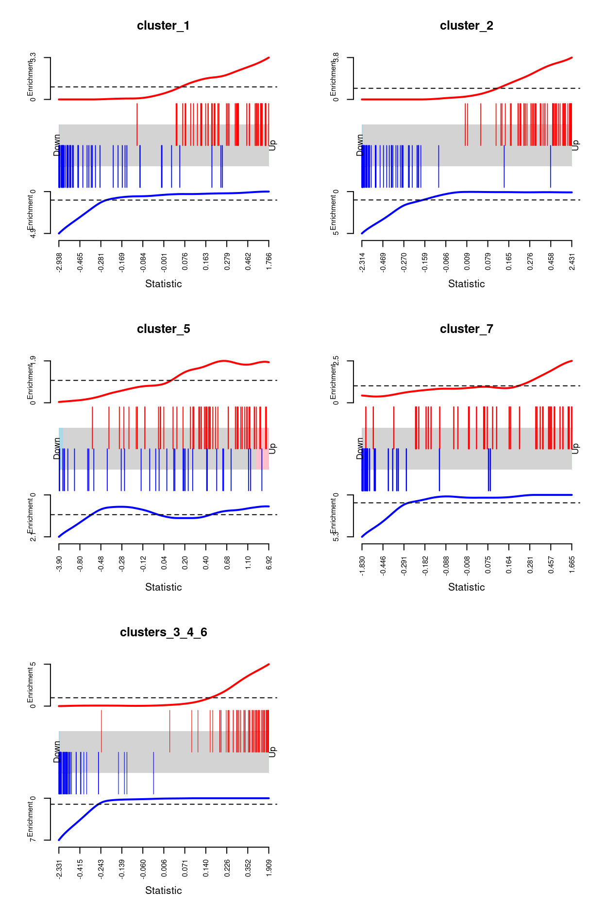
Figure 8: Barcode plot of the ignoring_clusters DEGs amongst the within-label DE analyses. An enrichment line shows the relative enrichment of the vertical bars in each part of the plot is displayed.
Comments on interpretation
DA or DE? Two sides of the same coin
While useful, the distinction between DA and DE analyses is inherently artificial for scRNA-seq data. This is because the labels used in the former are defined based on the genes to be tested in the latter. To illustrate, consider a scRNA-seq experiment involving two biological conditions with several shared cell types. We focus on a cell type \(X\) that is present in both conditions but contains some DEGs between conditions. This leads to two possible outcomes:
- The DE between conditions causes \(X\) to form two separate clusters (say, \(X_1\) and \(X_2\) in expression space. This manifests as DA where \(X_1\) is enriched in one condition and \(X_2\) is enriched in the other condition.
- The DE between conditions is not sufficient to split \(X\) into two separate clusters, e.g., because the data integration procedure identifies them as corresponding cell types and merges them together. This means that the differences between conditions manifest as DE within the single cluster corresponding to \(X\).
We have described the example above in terms of clustering, but the same arguments apply for any labelling strategy based on the expression profiles, e.g., automated cell type assignment. Moreover, the choice between outcomes 1 and 2 is made implicitly by the combined effect of the data merging, clustering and label assignment procedures. For example, differences between conditions are more likely to manifest as DE for coarser clusters and as DA for finer clusters, but this is difficult to predict reliably.
The moral of the story is that DA and DE analyses are simply two different perspectives on the same phenomena. For any comprehensive characterization of differences between populations, it is usually necessary to consider both analyses. Indeed, they complement each other almost by definition, e.g., clustering parameters that reduce DE will increase DA and vice versa.
Additional information
The following are available on request:
- Full CSV tables of any data presented.
- PDF/PNG files of any static plots.
Session info
─ Session info ─────────────────────────────────────────────────────
 setting  value
 version  R version 4.0.0 (2020-04-24)
 os       CentOS Linux 7 (Core)
 system   x86_64, linux-gnu
 ui       X11
 language (EN)
 collate  en_US.UTF-8
 ctype    en_US.UTF-8
 tz       Australia/Melbourne
 date     2020-10-01

─ Packages ─────────────────────────────────────────────────────────
 ! package              * version  date       lib source
 P AnnotationDbi        * 1.50.1   2020-06-29 [?] Bioconductor
 P assertthat             0.2.1    2019-03-21 [?] CRAN (R 4.0.0)
 P backports              1.1.8    2020-06-17 [?] CRAN (R 4.0.0)
 P beeswarm               0.2.3    2016-04-25 [?] CRAN (R 4.0.0)
 P Biobase              * 2.48.0   2020-04-27 [?] Bioconductor
 P BiocGenerics         * 0.34.0   2020-04-27 [?] Bioconductor
 P BiocManager            1.30.10  2019-11-16 [?] CRAN (R 4.0.0)
 P BiocNeighbors          1.6.0    2020-04-27 [?] Bioconductor
 P BiocParallel         * 1.22.0   2020-04-27 [?] Bioconductor
 P BiocSingular           1.4.0    2020-04-27 [?] Bioconductor
 P BiocStyle              2.16.0   2020-04-27 [?] Bioconductor
 P bit                    1.1-15.2 2020-02-10 [?] CRAN (R 4.0.0)
 P bit64                  0.9-7.1  2020-07-15 [?] CRAN (R 4.0.0)
 P bitops                 1.0-6    2013-08-17 [?] CRAN (R 4.0.0)
 P blob                   1.2.1    2020-01-20 [?] CRAN (R 4.0.0)
 P cellranger             1.1.0    2016-07-27 [?] CRAN (R 4.0.0)
 P cli                    2.0.2    2020-02-28 [?] CRAN (R 4.0.0)
 P colorspace             1.4-1    2019-03-18 [?] CRAN (R 4.0.0)
 P cowplot              * 1.0.0    2019-07-11 [?] CRAN (R 4.0.0)
 P crayon                 1.3.4    2017-09-16 [?] CRAN (R 4.0.0)
 P DBI                    1.1.0    2019-12-15 [?] CRAN (R 4.0.0)
 P DelayedArray         * 0.14.1   2020-07-14 [?] Bioconductor
 P DelayedMatrixStats     1.10.1   2020-07-03 [?] Bioconductor
 P digest                 0.6.25   2020-02-23 [?] CRAN (R 4.0.0)
 P distill                0.8      2020-06-04 [?] CRAN (R 4.0.0)
 P dplyr                  1.0.0    2020-05-29 [?] CRAN (R 4.0.0)
 P dqrng                  0.2.1    2019-05-17 [?] CRAN (R 4.0.0)
 P edgeR                * 3.30.3   2020-06-02 [?] Bioconductor
 P ellipsis               0.3.1    2020-05-15 [?] CRAN (R 4.0.0)
 P evaluate               0.14     2019-05-28 [?] CRAN (R 4.0.0)
 P fansi                  0.4.1    2020-01-08 [?] CRAN (R 4.0.0)
 P farver                 2.0.3    2020-01-16 [?] CRAN (R 4.0.0)
 P generics               0.0.2    2018-11-29 [?] CRAN (R 4.0.0)
 P GenomeInfoDb         * 1.24.2   2020-06-15 [?] Bioconductor
 P GenomeInfoDbData       1.2.3    2020-05-18 [?] Bioconductor
 P GenomicRanges        * 1.40.0   2020-04-27 [?] Bioconductor
 P ggbeeswarm             0.6.0    2017-08-07 [?] CRAN (R 4.0.0)
 P ggplot2              * 3.3.2    2020-06-19 [?] CRAN (R 4.0.0)
 P Glimma                 1.16.0   2020-04-27 [?] Bioconductor
 P glue                   1.4.1    2020-05-13 [?] CRAN (R 4.0.0)
 P GO.db                  3.11.4   2020-07-15 [?] Bioconductor
 P gridExtra              2.3      2017-09-09 [?] CRAN (R 4.0.0)
 P gtable                 0.3.0    2019-03-25 [?] CRAN (R 4.0.0)
 P here                 * 0.1      2017-05-28 [?] CRAN (R 4.0.0)
 P highr                  0.8      2019-03-20 [?] CRAN (R 4.0.0)
 P htmltools              0.5.0    2020-06-16 [?] CRAN (R 4.0.0)
 P igraph                 1.2.5    2020-03-19 [?] CRAN (R 4.0.0)
 P IRanges              * 2.22.2   2020-05-21 [?] Bioconductor
 P irlba                  2.3.3    2019-02-05 [?] CRAN (R 4.0.0)
 P jsonlite               1.7.0    2020-06-25 [?] CRAN (R 4.0.0)
 P knitr                  1.29     2020-06-23 [?] CRAN (R 4.0.0)
 P labeling               0.3      2014-08-23 [?] CRAN (R 4.0.0)
 P lattice                0.20-41  2020-04-02 [?] CRAN (R 4.0.0)
 P lifecycle              0.2.0    2020-03-06 [?] CRAN (R 4.0.0)
 P limma                * 3.44.3   2020-06-12 [?] Bioconductor
 P locfit                 1.5-9.4  2020-03-25 [?] CRAN (R 4.0.0)
 P magrittr               1.5      2014-11-22 [?] CRAN (R 4.0.0)
 P Matrix                 1.2-18   2019-11-27 [?] CRAN (R 4.0.0)
 P matrixStats          * 0.56.0   2020-03-13 [?] CRAN (R 4.0.0)
 P memoise                1.1.0    2017-04-21 [?] CRAN (R 4.0.0)
 P msigdbr              * 7.1.1    2020-05-14 [?] CRAN (R 4.0.0)
 P munsell                0.5.0    2018-06-12 [?] CRAN (R 4.0.0)
 P org.Mm.eg.db         * 3.11.4   2020-06-02 [?] Bioconductor
 P patchwork            * 1.0.1    2020-06-22 [?] CRAN (R 4.0.0)
 P pheatmap             * 1.0.12   2019-01-04 [?] CRAN (R 4.0.0)
 P pillar                 1.4.6    2020-07-10 [?] CRAN (R 4.0.0)
 P pkgconfig              2.0.3    2019-09-22 [?] CRAN (R 4.0.0)
 P purrr                  0.3.4    2020-04-17 [?] CRAN (R 4.0.0)
 P R6                     2.4.1    2019-11-12 [?] CRAN (R 4.0.0)
 P RColorBrewer           1.1-2    2014-12-07 [?] CRAN (R 4.0.0)
 P Rcpp                   1.0.5    2020-07-06 [?] CRAN (R 4.0.0)
 P RCurl                  1.98-1.2 2020-04-18 [?] CRAN (R 4.0.0)
 P readxl                 1.3.1    2019-03-13 [?] CRAN (R 4.0.0)
 P rlang                  0.4.7    2020-07-09 [?] CRAN (R 4.0.0)
 P rmarkdown              2.3      2020-06-18 [?] CRAN (R 4.0.0)
 P rprojroot              1.3-2    2018-01-03 [?] CRAN (R 4.0.0)
 P RSQLite                2.2.0    2020-01-07 [?] CRAN (R 4.0.0)
 P rsvd                   1.0.3    2020-02-17 [?] CRAN (R 4.0.0)
 P S4Vectors            * 0.26.1   2020-05-16 [?] Bioconductor
 P scales                 1.1.1    2020-05-11 [?] CRAN (R 4.0.0)
 P scater               * 1.16.2   2020-06-26 [?] Bioconductor
 P scran                * 1.16.0   2020-04-27 [?] Bioconductor
 P sessioninfo            1.1.1    2018-11-05 [?] CRAN (R 4.0.0)
 P SingleCellExperiment * 1.10.1   2020-04-28 [?] Bioconductor
 P statmod                1.4.34   2020-02-17 [?] CRAN (R 4.0.0)
 P stringi                1.4.6    2020-02-17 [?] CRAN (R 4.0.0)
 P stringr                1.4.0    2019-02-10 [?] CRAN (R 4.0.0)
 P SummarizedExperiment * 1.18.2   2020-07-09 [?] Bioconductor
 P tibble                 3.0.3    2020-07-10 [?] CRAN (R 4.0.0)
 P tidyr                  1.1.0    2020-05-20 [?] CRAN (R 4.0.0)
 P tidyselect             1.1.0    2020-05-11 [?] CRAN (R 4.0.0)
 P vctrs                  0.3.2    2020-07-15 [?] CRAN (R 4.0.0)
 P vipor                  0.4.5    2017-03-22 [?] CRAN (R 4.0.0)
 P viridis                0.5.1    2018-03-29 [?] CRAN (R 4.0.0)
 P viridisLite            0.3.0    2018-02-01 [?] CRAN (R 4.0.0)
 P withr                  2.2.0    2020-04-20 [?] CRAN (R 4.0.0)
 P xfun                   0.15     2020-06-21 [?] CRAN (R 4.0.0)
 P XVector                0.28.0   2020-04-27 [?] Bioconductor
 P yaml                   2.2.1    2020-02-01 [?] CRAN (R 4.0.0)
 P zlibbioc               1.34.0   2020-04-27 [?] Bioconductor

[1] /stornext/General/data/user_managed/grpu_mritchie_1/hickey/SCORE/C075_Grant_Coultas/renv/library/R-4.0/x86_64-pc-linux-gnu
[2] /tmp/RtmpCHylYX/renv-system-library
[3] /stornext/System/data/apps/R/R-4.0.0/lib64/R/library

 P ── Loaded and on-disk path mismatch.
Chen, Y., A. T. L. Lun, and G. K. Smyth. 2014. “Differential Expression Analysis of Complex Rna-Seq Experiments Using edgeR.” In Statistical Analysis of Next Generation Sequencing Data, edited by S. Datta and D. Nettleton, 51–74. Springer.
Crowell, H. L., C. Soneson, P.-L. Germain, D. Calini, L. Collin, C. Raposo, D. Malhotra, and M. D. Robinson. 2019. “On the Discovery of Population-Specific State Transitions from Multi-Sample Multi-Condition Single-Cell Rna Sequencing Data.” bioRxiv. https://doi.org/10.1101/713412.
Finak, G., A. McDavid, M. Yajima, J. Deng, V. Gersuk, A. K. Shalek, C. K. Slichter, et al. 2015. “MAST: A Flexible Statistical Framework for Assessing Transcriptional Changes and Characterizing Heterogeneity in Single-Cell Rna Sequencing Data.” Genome Biol. 16: 278.
Lun, Aaron TL, and John C Marioni. 2017. “Overcoming Confounding Plate Effects in Differential Expression Analyses of Single-Cell Rna-Seq Data.” Biostatistics 18 (3): 451–64.
Lun, A. T. L., A. C. Richard, and J. C. Marioni. 2017. “Testing for Differential Abundance in Mass Cytometry Data.” Nat. Methods 14 (7): 707–9.
Richard, A. C., A. T. L. Lun, W. W. Y. Lau, B. Gottgens, J. C. Marioni, and G. M. Griffiths. 2018. “T Cell Cytolytic Capacity Is Independent of Initial Stimulation Strength.” Nat. Immunol. 19 (8): 849–58.
Robinson, M. D., D. J. McCarthy, and G. K. Smyth. 2010. “EdgeR: A Bioconductor Package for Differential Expression Analysis of Digital Gene Expression Data.” Bioinformatics 26 (1): 139–40.
Robinson, M. D., and A. Oshlack. 2010. “A Scaling Normalization Method for Differential Expression Analysis of Rna-Seq Data.” Genome Biol. 11 (3): R25. https://www.ncbi.nlm.nih.gov/pubmed/20196867.
Scialdone, A., Y. Tanaka, W. Jawaid, V. Moignard, N. K. Wilson, I. C. Macaulay, J. C. Marioni, and B. Gottgens. 2016. “Resolving Early Mesoderm Diversification Through Single-Cell Expression Profiling.” Nature 535 (7611): 289–93.
Tung, P. Y., J. D. Blischak, C. J. Hsiao, D. A. Knowles, J. E. Burnett, J. K. Pritchard, and Y. Gilad. 2017. “Batch Effects and the Effective Design of Single-Cell Gene Expression Studies.” Sci. Rep. 7 (January): 39921.
Wu, Di, Elgene Lim, François Vaillant, Marie-Liesse Asselin-Labat, Jane E Visvader, and Gordon K Smyth. 2010. “ROAST: Rotation Gene Set Tests for Complex Microarray Experiments.” Bioinformatics 26 (17): 2176–82.
In estimating both the NB and QL dispersion we turn off the trend estimation as we do not have enough points for its stable estimation↩︎
E.g., the saddlepoint approximation for quasi-likelihood methods or normality for linear models.↩︎
A mixed effects model can handle this variance structure but involves extra statistical and computational complexity for little benefit, see Crowell et al.↩︎
Of course, high per-cell variability will still result in weaker DE if it affects the variability across populations, while homogeneous per-cell responses will result in stronger DE due to a larger population-level log-fold change. These effects are also largely desirable.↩︎
E.g., Crowell et al. note that “\(\approx100\) cells is sufficient to reach decent performance” with pseudobulk DE methods and that “there is a sizable gain in performance in going from 50 to 100 cells” per label per sample.↩︎
Please note that these results do not take into account the directionality of the log-fold change.↩︎
Please note that these results do not take into account the directionality of the log-fold change.↩︎
Note that the number of
UpandDowngenes may not match the number of entires inupGeneSymbolsanddownGeneSymbolin these spreadsheets. This is because we have performed our analysis using the Ensembl gene ID as the features whereas the GO and KEGG analyses using Entrez gene IDs. There is no one-to-one mapping between the Ensembl gene IDs, Entrez gene IDs, and NCBI gene symbols, which leads to the slight variations of the gene numbers in these spreadsheets.↩︎