Setup
Show code
library(SingleCellExperiment)
library(here)
library(cowplot)
library(patchwork)

sce <- readRDS(here("data/SCEs/C057_Cooney.cells_selected.SCE.rds"))

# data frames containing co-ordinates and factors for creating reduced
# dimensionality plots.
umap_df <- cbind(
  data.frame(
    x = reducedDim(sce, "UMAP")[, 1],
    y = reducedDim(sce, "UMAP")[, 2]),
  as.data.frame(colData(sce)[, !colnames(colData(sce)) %in% c("TRA", "TRB")]))

# Some useful colours
sample_colours <- setNames(
  unique(sce$sample_colours),
  unique(names(sce$sample_colours)))
treatment_colours <- setNames(
  unique(sce$treatment_colours),
  unique(names(sce$treatment_colours)))
cluster_colours <- setNames(
  unique(sce$cluster_colours),
  unique(names(sce$cluster_colours)))

# Some useful gene sets
mito_set <- rownames(sce)[which(rowData(sce)$CHR == "MT")]
ribo_set <- grep("^RP(S|L)", rownames(sce), value = TRUE)
# NOTE: A more curated approach for identifying ribosomal protein genes
#       (https://github.com/Bioconductor/OrchestratingSingleCellAnalysis-base/blob/ae201bf26e3e4fa82d9165d8abf4f4dc4b8e5a68/feature-selection.Rmd#L376-L380)
library(msigdbr)
c2_sets <- msigdbr(species = "Homo sapiens", category = "C2")
ribo_set <- union(
  ribo_set,
  c2_sets[c2_sets$gs_name == "KEGG_RIBOSOME", ]$human_gene_symbol)

source(here("code", "helper_functions.R"))
Re-processing
This is a no-op if the same hvg set is used from cell selection.
Show code
library(scran)
set.seed(1000)
var_fit <- modelGeneVarByPoisson(sce, block = sce$batch)
hvg <- getTopHVGs(var_fit, var.threshold = 0)
is_mito <- hvg %in% mito_set
is_ribo <- hvg %in% ribo_set
hvg <- hvg[!(is_mito | is_ribo)]

set.seed(1010)
var_fit.sample <- modelGeneVarByPoisson(sce, block = sce$Sample)
hvg.sample <- getTopHVGs(var_fit.sample, var.threshold = 0)
is_mito <- hvg.sample %in% mito_set
is_ribo <- hvg.sample %in% ribo_set
hvg.sample <- hvg.sample[!(is_mito | is_ribo)]

library(scater)
# NOTE:
set.seed(11235)
sce <- denoisePCA(sce, var_fit, subset.row = hvg)
set.seed(8875)
sce <- runUMAP(sce, dimred = "PCA")
umap_df <- cbind(
  data.frame(
    x = reducedDim(sce, "UMAP")[, 1],
    y = reducedDim(sce, "UMAP")[, 2]),
  as.data.frame(colData(sce)[, !colnames(colData(sce)) %in% c("TRA", "TRB")]))
set.seed(8111)
snn_gr <- buildSNNGraph(sce, use.dimred = "PCA")
clusters <- igraph::cluster_louvain(snn_gr)
sce$cluster <- factor(clusters$membership)
umap_df$cluster <- sce$cluster
cluster_colours <- setNames(
  Polychrome::glasbey.colors(nlevels(sce$cluster) + 1)[-1],
  levels(sce$cluster))
sce$cluster_colours <- cluster_colours[sce$cluster]
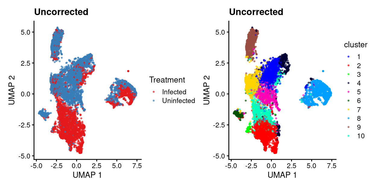
Diagnosing batch effects
- Samples were collected in a single capture, but there are some strong differences between Venetoclax and Control samples.
- Explore whether batch effect exists and how it might be corrected.
Show code
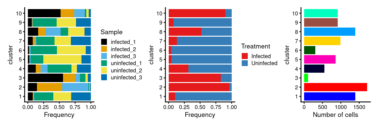
table(cluster = sce$cluster, treatment = sce$Treatment)
       treatment
cluster Infected Uninfected
     1       141       1248
     2      1651         66
     3        86         18
     4       173        379
     5        37        816
     6        13        291
     7       133        856
     8       724        671
     9        71        840
     10      827         90
Show code
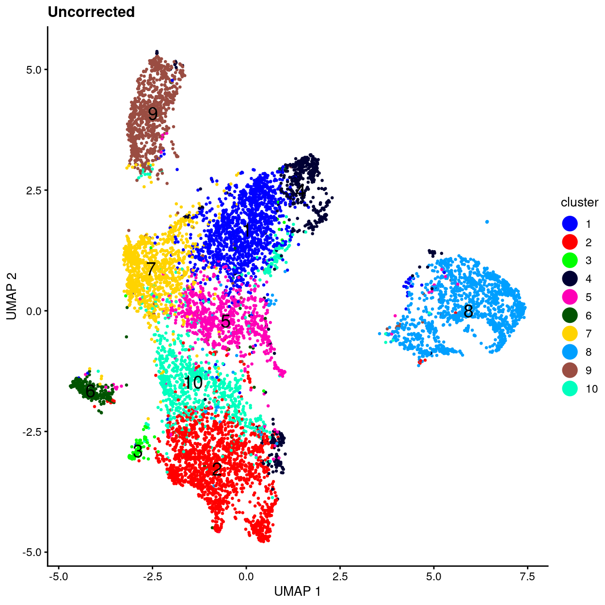
uncorrected.p1 <- plotUMAP(sce, colour_by = "Treatment", point_size = 0.5) +
  scale_colour_manual(values = treatment_colours, name = "Treatment") +
  ggtitle("Uncorrected")
uncorrected.p2 <- plotUMAP(sce, colour_by = "cluster", point_size = 0.5) +
  scale_colour_manual(values = cluster_colours, name = "cluster") +
  ggtitle("Uncorrected")
uncorrected.p1 + uncorrected.p2
Show code
p1 <- ggplot(as.data.frame(colData(sce)[, c("cluster", "Sample")])) +
  geom_bar(
    aes(x = cluster, fill = Sample),
    position = position_fill(reverse = TRUE)) +
  coord_flip() +
  ylab("Frequency") +
  scale_fill_manual(values = sample_colours) +
  theme_cowplot(font_size = 8)
p2 <- ggplot(as.data.frame(colData(sce)[, c("cluster", "Treatment")])) +
  geom_bar(
    aes(x = cluster, fill = Treatment),
    position = position_fill(reverse = TRUE)) +
  coord_flip() +
  ylab("Frequency") +
  scale_fill_manual(values = treatment_colours) +
  theme_cowplot(font_size = 8)
p3 <- ggplot(as.data.frame(colData(sce)[, "cluster", drop = FALSE])) +
  geom_bar(aes(x = cluster, fill = cluster)) +
  coord_flip() +
  ylab("Number of cells") +
  scale_fill_manual(values = cluster_colours) +
  theme_cowplot(font_size = 8) +
  guides(fill = FALSE)
p1 + p2 + p3
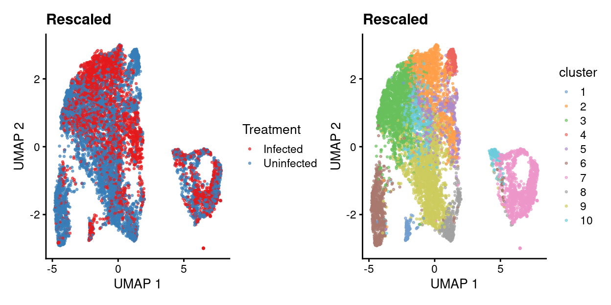
Linear regression with rescaleBatches()
Show code
library(batchelor)
rescaled <- rescaleBatches(sce, batch = sce$Treatment)
library(scran)
set.seed(666)
rescaled <- denoisePCA(
rescaled,
var_fit,
subset.row = hvg,
assay.type = "corrected")
snn.gr <- buildSNNGraph(rescaled, use.dimred="PCA")
clusters.resc <- igraph::cluster_louvain(snn.gr)$membership
rescaled <- runUMAP(rescaled, dimred="PCA")
rescaled$batch <- factor(rescaled$batch)
rescaled$cluster <- factor(clusters.resc)
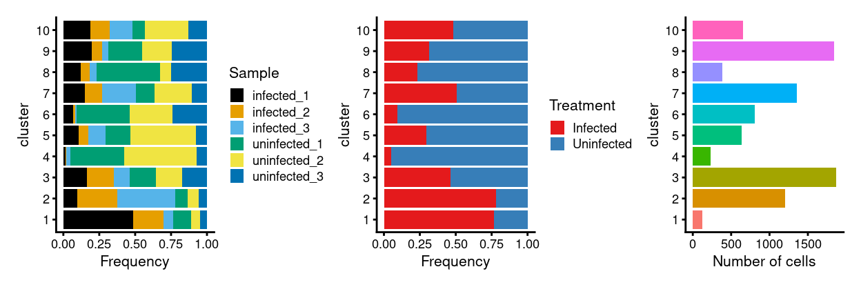
table(cluster=clusters.resc, treatment=rescaled$batch)
       treatment
cluster Infected Uninfected
     1        98         30
     2       942        264
     3       868       1004
     4        12        223
     5       189        450
     6        76        735
     7       687        672
     8        89        295
     9       579       1264
     10      316        338
Show code
Show code
p1 <- ggplot(as.data.frame(
  cbind(
    colData(sce)[, "Sample", drop = FALSE],
    colData(rescaled)[, "cluster", drop = FALSE]))) +
  geom_bar(
    aes(x = cluster, fill = Sample),
    position = position_fill(reverse = TRUE)) +
  coord_flip() +
  ylab("Frequency") +
    scale_fill_manual(values = sample_colours) +
    theme_cowplot(font_size = 8)
p2 <- ggplot(as.data.frame(
    cbind(
      colData(sce)[, "Treatment", drop = FALSE],
      colData(rescaled)[, "cluster", drop = FALSE]))) +
    geom_bar(
      aes(x = cluster, fill = Treatment),
      position = position_fill(reverse = TRUE)) +
    coord_flip() +
    ylab("Frequency") +
    scale_fill_manual(values = treatment_colours) +
    theme_cowplot(font_size = 8)
p3 <- ggplot(as.data.frame(colData(rescaled)[, "cluster", drop = FALSE])) +
  geom_bar(aes(x = cluster, fill = cluster)) +
  coord_flip() +
  ylab("Number of cells") +
  theme_cowplot(font_size = 8) +
  guides(fill = FALSE)
p1 + p2 + p3
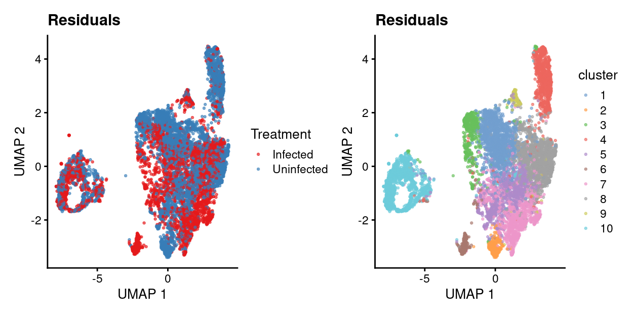
Linear regression with regressBatches()
Show code
set.seed(10001)
residuals <- regressBatches(sce, batch = sce$Treatment, d = 50,
                            subset.row=hvg, correct.all=TRUE)

snn.gr <- buildSNNGraph(residuals, use.dimred="corrected")
clusters.resid <- igraph::cluster_louvain(snn.gr)$membership
table(Cluster=clusters.resid, treatment=residuals$batch)
       treatment
Cluster Infected Uninfected
     1       519       1168
     2        19        254
     3       191        380
     4        92        817
     5       195        814
     6       249          7
     7      1031        223
     8       740        884
     9        91         28
     10      729        700
Show code
residuals <- runUMAP(residuals, dimred="corrected")
residuals$batch <- factor(residuals$batch)
residuals$cluster <- factor(clusters.resid)
residuals.p1 <- plotUMAP(residuals, colour_by = "batch", point_size = 0.5) +
  scale_colour_manual(values = treatment_colours, name = "Treatment") +
  ggtitle("Residuals")
residuals.p2 <- plotUMAP(residuals, colour_by = "cluster", point_size = 0.5) +
  ggtitle("Residuals")
residuals.p1 + residuals.p2
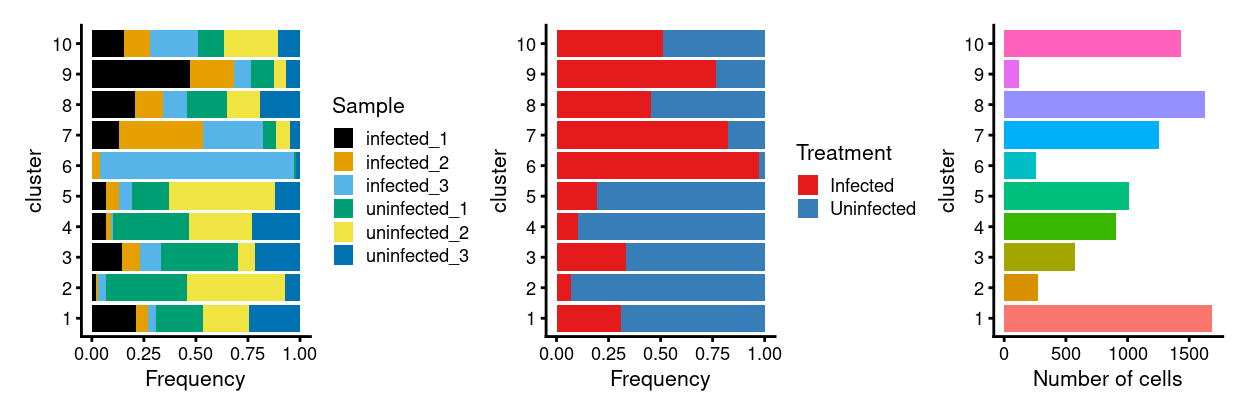
Show code
p1 <- ggplot(as.data.frame(
    cbind(
      colData(sce)[, "Sample", drop = FALSE],
      colData(residuals)[, "cluster", drop = FALSE]))) +
    geom_bar(
      aes(x = cluster, fill = Sample),
      position = position_fill(reverse = TRUE)) +
    coord_flip() +
    ylab("Frequency") +
    scale_fill_manual(values = sample_colours) +
    theme_cowplot(font_size = 8)
p2 <- ggplot(as.data.frame(
    cbind(
      colData(sce)[, "Treatment", drop = FALSE],
      colData(residuals)[, "cluster", drop = FALSE]))) +
    geom_bar(
      aes(x = cluster, fill = Treatment),
      position = position_fill(reverse = TRUE)) +
    coord_flip() +
    ylab("Frequency") +
    scale_fill_manual(values = treatment_colours) +
    theme_cowplot(font_size = 8)
p3 <- ggplot(as.data.frame(colData(residuals)[, "cluster", drop = FALSE])) +
    geom_bar(aes(x = cluster, fill = cluster)) +
    coord_flip() +
    ylab("Number of cells") +
    theme_cowplot(font_size = 8) +
    guides(fill = FALSE)
p1 + p2 + p3
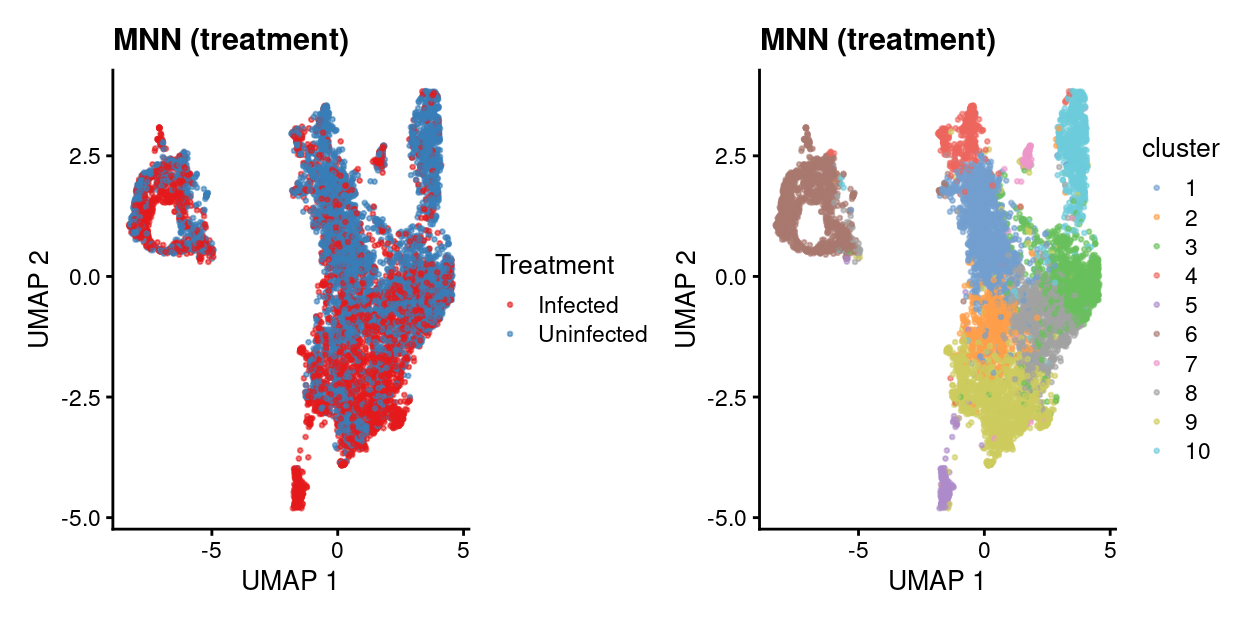
MNN by treatment
Show code
set.seed(1000101001)
mnn_treatment.out <- fastMNN(
  sce,
  batch = sce$Treatment,
  d = 50,
  k = 20,
  subset.row = hvg)
snn.gr <- buildSNNGraph(mnn_treatment.out, use.dimred="corrected")
clusters.mnn_treatment <- igraph::cluster_louvain(snn.gr)$membership
table(Cluster=clusters.mnn_treatment, treatment=mnn_treatment.out$batch)
       treatment
Cluster Infected Uninfected
     1       341       1245
     2       270        308
     3       327        802
     4       110        336
     5       239          4
     6       710        679
     7        67         28
     8       521        572
     9      1179        577
     10       92        724
Show code
mnn_treatment.out <- runUMAP(mnn_treatment.out, dimred="corrected")
mnn_treatment.out$batch <- factor(mnn_treatment.out$batch)
mnn_treatment.out$cluster <- factor(clusters.mnn_treatment)
mnn_treatment.p1 <- plotUMAP(
  mnn_treatment.out,
  colour_by = "batch",
  point_size = 0.5) +
  scale_colour_manual(values = treatment_colours, name = "Treatment") +
  ggtitle("MNN (treatment)")
mnn_treatment.p2 <- plotUMAP(
  mnn_treatment.out,
  colour_by = "cluster",
  point_size = 0.5) +
  ggtitle("MNN (treatment)")
mnn_treatment.p1 + mnn_treatment.p2
Show code
metadata(mnn_treatment.out)$merge.info$lost.var
Infected Uninfected
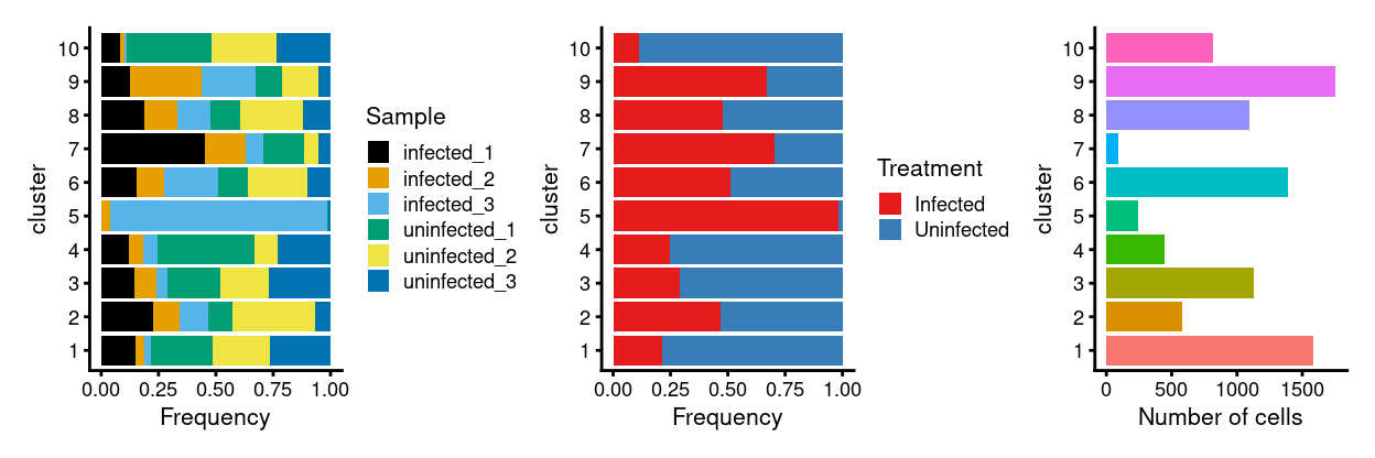
[1,] 0.02292624 0.0100355Show code
p1 <- ggplot(as.data.frame(
    cbind(
      colData(sce)[, "Sample", drop = FALSE],
      colData(mnn_treatment.out)[, "cluster", drop = FALSE]))) +
    geom_bar(
      aes(x = cluster, fill = Sample),
      position = position_fill(reverse = TRUE)) +
    coord_flip() +
    ylab("Frequency") +
    scale_fill_manual(values = sample_colours) +
    theme_cowplot(font_size = 8)
p2 <- ggplot(as.data.frame(
    cbind(
      colData(sce)[, "Treatment", drop = FALSE],
      colData(mnn_treatment.out)[, "cluster", drop = FALSE]))) +
    geom_bar(
      aes(x = cluster, fill = Treatment),
      position = position_fill(reverse = TRUE)) +
    coord_flip() +
    ylab("Frequency") +
    scale_fill_manual(values = treatment_colours) +
    theme_cowplot(font_size = 8)
p3 <- ggplot(
  as.data.frame(colData(mnn_treatment.out)[, "cluster", drop = FALSE])) +
  geom_bar(aes(x = cluster, fill = cluster)) +
  coord_flip() +
  ylab("Number of cells") +
  theme_cowplot(font_size = 8) +
  guides(fill = FALSE)
p1 + p2 + p3
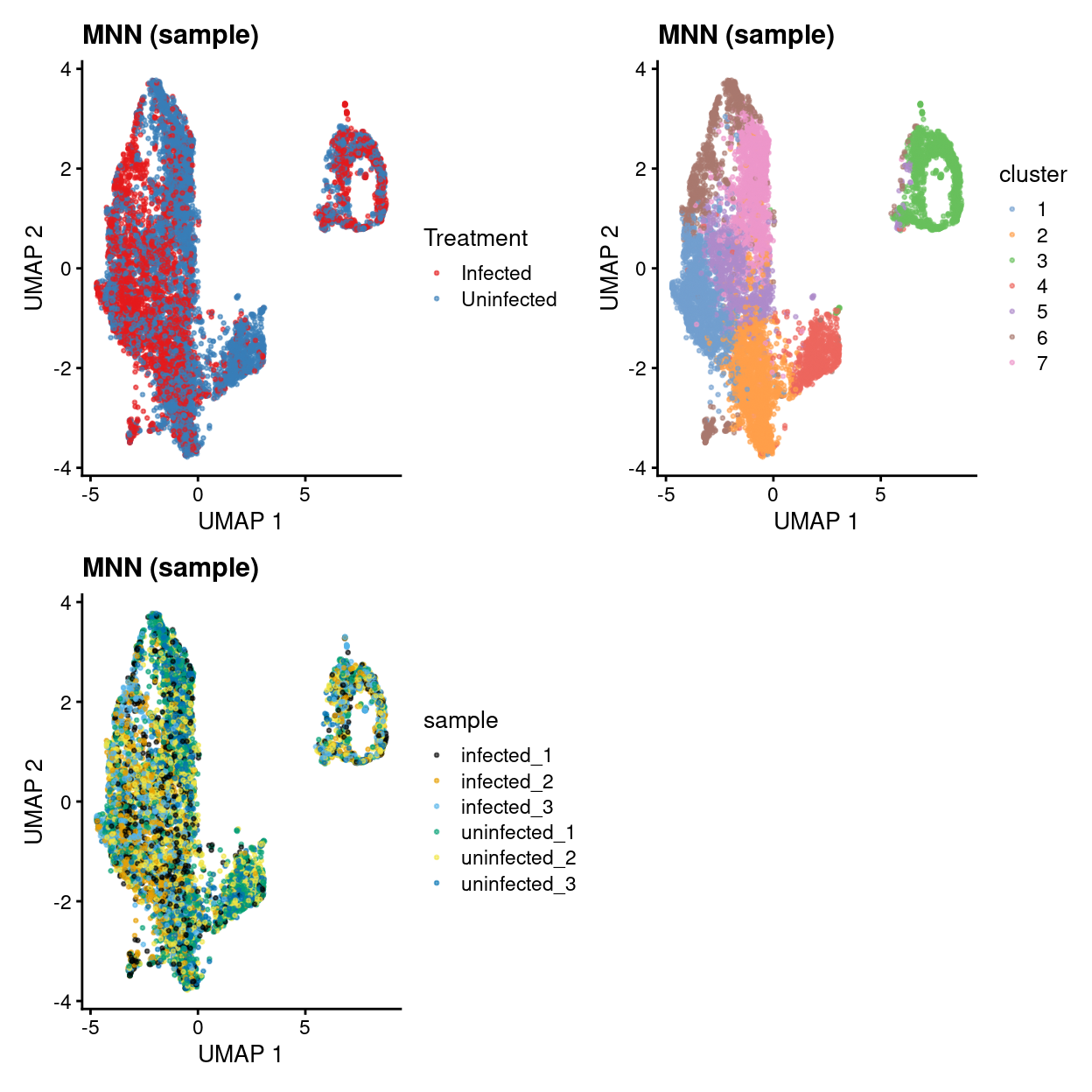
MNN by sample
Show code
set.seed(1000101001)
mnn_sample.out <- fastMNN(
  sce,
  batch = sce$Sample,
  d = 50,
  k = 20,
  subset.row = hvg.sample)
snn.gr <- buildSNNGraph(mnn_sample.out, use.dimred="corrected")
clusters.mnn_sample <- igraph::cluster_louvain(snn.gr)$membership
table(Cluster = clusters.mnn_sample, treatment = mnn_sample.out$batch)
       treatment
Cluster infected_1 infected_2 infected_3 uninfected_1 uninfected_2
      1        205        366        383          202          254
      2        281        260        182          378          406
      3        208        164        327          181          348
      4         60         16          9          280          226
      5        193        166        207          116          299
      6        169        132        171          242          132
      7        231         71         55          390          387
       treatment
Cluster uninfected_3
      1           98
      2          359
      3          140
      4          196
      5           93
      6          132
      7          416
Show code
mnn_sample.out <- runUMAP(mnn_sample.out, dimred="corrected")
mnn_sample.out$batch <- factor(mnn_sample.out$batch)
mnn_sample.out$cluster <- factor(clusters.mnn_sample)
mnn_sample.p1 <- plotUMAP(
  mnn_sample.out,
  colour_by = I(sce$Treatment),
  point_size = 0.5) +
  scale_colour_manual(values = treatment_colours, name = "Treatment") +
  ggtitle("MNN (sample)")
mnn_sample.p2 <- plotUMAP(
  mnn_sample.out,
  colour_by = "cluster",
  point_size = 0.5) +
  ggtitle("MNN (sample)")
mnn_sample.p3 <- plotUMAP(
  mnn_sample.out,
  colour_by = "batch",
  point_size = 0.5) +
  scale_colour_manual(values = sample_colours, name = "sample") +
  ggtitle("MNN (sample)")
mnn_sample.p1 + mnn_sample.p2 + mnn_sample.p3 + plot_layout(ncol = 2)
Show code
round(metadata(mnn_sample.out)$merge.info$lost.var, 3)
     infected_1 infected_2 infected_3 uninfected_1 uninfected_2
[1,]      0.021      0.034      0.000        0.000        0.000
[2,]      0.003      0.003      0.032        0.000        0.000
[3,]      0.016      0.012      0.010        0.029        0.000
[4,]      0.002      0.002      0.002        0.003        0.038
[5,]      0.002      0.002      0.002        0.003        0.003
     uninfected_3
[1,]        0.000
[2,]        0.000
[3,]        0.000
[4,]        0.000
[5,]        0.044
Show code
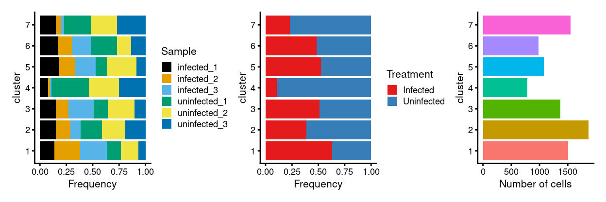
p1 <- ggplot(as.data.frame(
  cbind(
    colData(sce)[, "Sample", drop = FALSE],
    colData(mnn_sample.out)[, "cluster", drop = FALSE]))) +
  geom_bar(
    aes(x = cluster, fill = Sample),
    position = position_fill(reverse = TRUE)) +
  coord_flip() +
  ylab("Frequency") +
  scale_fill_manual(values = sample_colours) +
  theme_cowplot(font_size = 8)
p2 <- ggplot(as.data.frame(
    cbind(
      colData(sce)[, "Treatment", drop = FALSE],
      colData(mnn_sample.out)[, "cluster", drop = FALSE]))) +
    geom_bar(
      aes(x = cluster, fill = Treatment),
      position = position_fill(reverse = TRUE)) +
    coord_flip() +
    ylab("Frequency") +
    scale_fill_manual(values = treatment_colours) +
    theme_cowplot(font_size = 8)
p3 <- ggplot(
  as.data.frame(colData(mnn_sample.out)[, "cluster", drop = FALSE])) +
    geom_bar(aes(x = cluster, fill = cluster)) +
    coord_flip() +
    ylab("Number of cells") +
    theme_cowplot(font_size = 8) +
    guides(fill = FALSE)
p1 + p2 + p3 + plot_layout(ncol = 3)
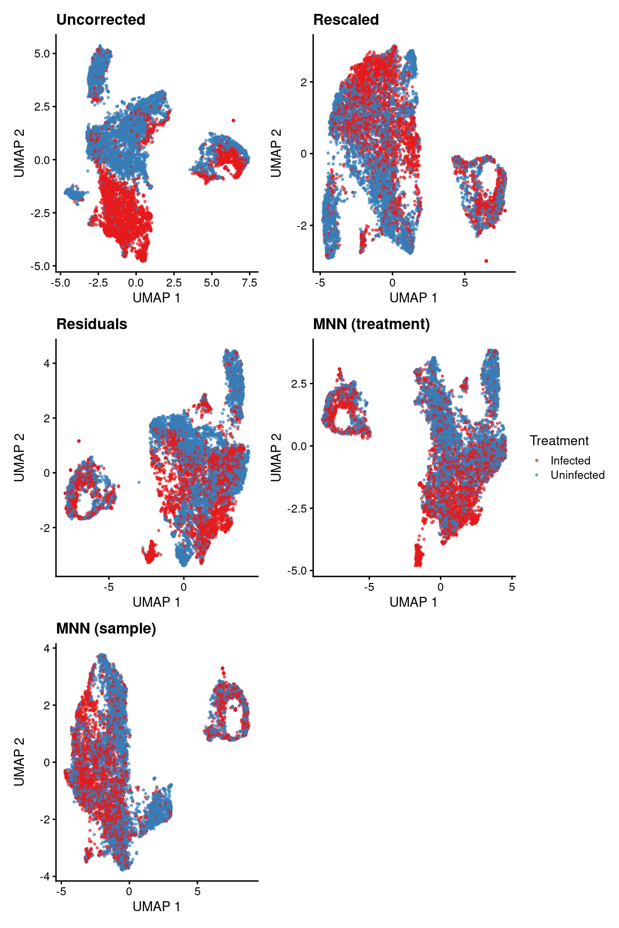
Summary of data integration results
Show code
uncorrected.p1 + rescaled.p1 + residuals.p1 + mnn_treatment.p1 +
  mnn_sample.p1 + plot_layout(ncol = 2, guides = "collect")
Show code
uncorrected.p2 + rescaled.p2 + residuals.p2 + mnn_treatment.p2 +
  mnn_sample.p2 + plot_layout(ncol = 2)
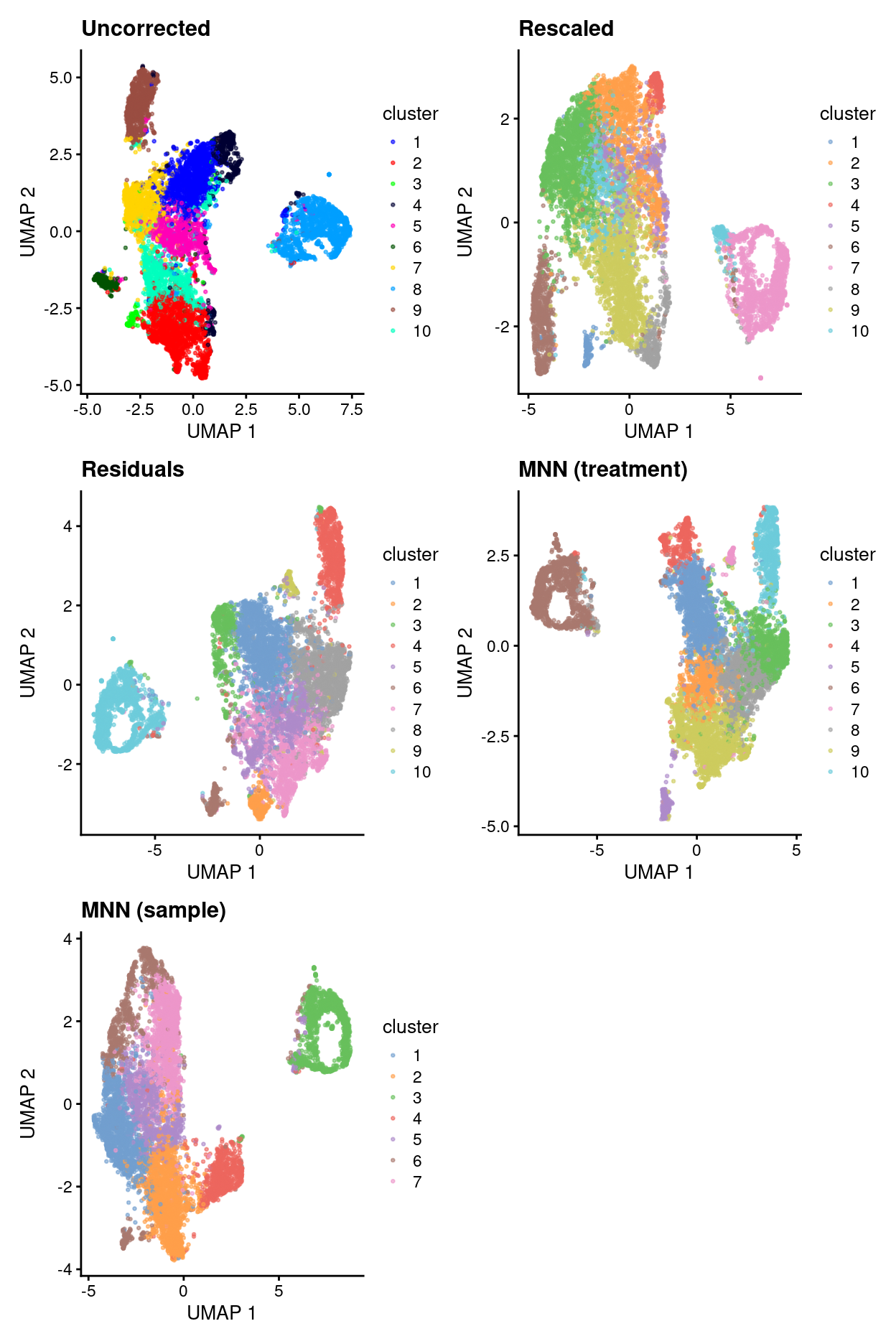
- Uncorrected data has strong treatment-specific differences (and presumably donor-specific differences).
- Correcting for treatment using any of the 4 approaches removes / dampens those treatment-specific differences.
- However, it’s a little hard to interpret if this is a good or bad thing.
- Therefore, will just use uncorrected data in what follows while remembering that this means there will be very treatment-specific (and perhaps donor-specific) clusters.
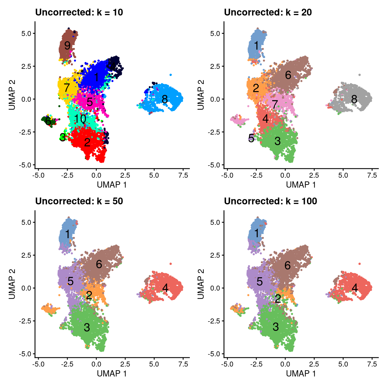
Clustering at different resolutions
- In all clusterings we observe an ‘out group’ on the right hand side.
Show code
set.seed(126)
snn_gr <- buildSNNGraph(sce, use.dimred = "PCA", k = 20)
clusters <- igraph::cluster_louvain(snn_gr)
sce$cluster_k20 <- factor(clusters$membership)
snn_gr <- buildSNNGraph(sce, use.dimred = "PCA", k = 50)
clusters <- igraph::cluster_louvain(snn_gr)
sce$cluster_k50 <- factor(clusters$membership)
snn_gr <- buildSNNGraph(sce, use.dimred = "PCA", k = 100)
clusters <- igraph::cluster_louvain(snn_gr)
sce$cluster_k100 <- factor(clusters$membership)

p1 <- plotUMAP(
  sce,
  colour_by = "cluster",
  point_size = 0.5,
  point_alpha = 1,
  text_by = "cluster") +
  scale_colour_manual(values = cluster_colours, name = "cluster") +
  ggtitle("Uncorrected: k = 10") +
  guides(colour = FALSE)
p2 <- plotUMAP(
  sce,
  colour_by = "cluster_k20",
  point_size = 0.5,
  point_alpha = 1,
  text_by = "cluster_k20") +
  ggtitle("Uncorrected: k = 20") +
  guides(colour = FALSE)
p3 <- plotUMAP(
  sce,
  colour_by = "cluster_k50",
  point_size = 0.5,
  point_alpha = 1,
  text_by = "cluster_k50") +
  ggtitle("Uncorrected: k = 50") +
  guides(colour = FALSE)
p4 <- plotUMAP(
  sce,
  colour_by = "cluster_k100",
  point_size = 0.5,
  point_alpha = 1,
  text_by = "cluster_k100") +
  ggtitle("Uncorrected: k = 100") +
  guides(colour = FALSE)
p1 + p2 + p3 + p4 + plot_layout(ncol = 2)
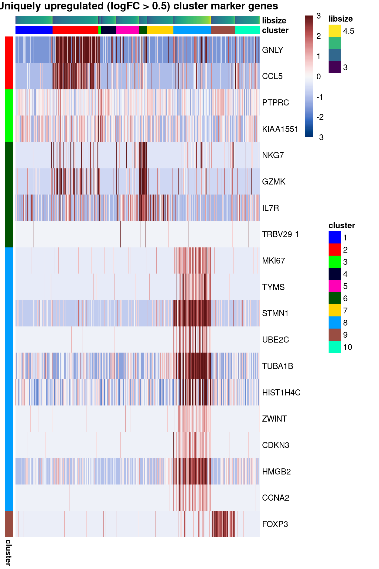
Some clusters are readily annotated by uniquely upregulated markers
Show code
Show code
# NOTE: Not blocking on `Sample` because some clusters are so `Sample`- and
#       `Treatment`-specific.
out <- pairwiseTTests(
  sce,
  sce$cluster,
  direction = "up",
  lfc = 0.5)
top_markers <- getTopMarkers(
  out$statistics,
  out$pairs,
  pairwise = FALSE,
  pval.type = "all")
features <- unlist(top_markers)
sce$libsize <- log10(sce$sum)
plotHeatmap(
  sce,
  features,
  order_columns_by = c("cluster", "libsize"),
  cluster_rows = FALSE,
  color = hcl.colors(101, "Blue-Red 3"),
  center = TRUE,
  zlim = c(-3, 3),
  column_annotation_colors = list(
    cluster = cluster_colours),
  annotation_row = data.frame(
    cluster = names(features),
    row.names = features),
  main = "Uniquely upregulated (logFC > 0.5) cluster marker genes")
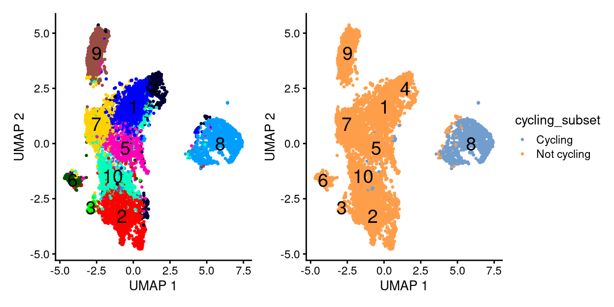
Cell cycle / proliferation of activated T-cells
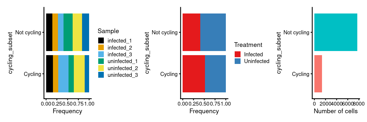
- There appears to be a cycling and non-cycling subset of clusters driving the initial clustering (cluster 8)
- Cycling subset typified by upregulation of a large number of genes, larger library sizes, and cyclin expression
- Cell cycle could really be proliferation of T-cells upon activation
Show code
Show code
p1 <- ggplot(as.data.frame(colData(sce)[, c("cycling_subset", "Sample")])) +
    geom_bar(
      aes(x = cycling_subset, fill = Sample),
      position = position_fill(reverse = TRUE)) +
    coord_flip() +
    ylab("Frequency") +
    scale_fill_manual(values = sample_colours) +
    theme_cowplot(font_size = 8)
p2 <- ggplot(as.data.frame(colData(sce)[, c("cycling_subset", "Treatment")])) +
    geom_bar(
      aes(x = cycling_subset, fill = Treatment),
      position = position_fill(reverse = TRUE)) +
    coord_flip() +
    ylab("Frequency") +
    scale_fill_manual(values = treatment_colours) +
    theme_cowplot(font_size = 8)
p3 <- ggplot(as.data.frame(colData(sce)[, "cycling_subset", drop = FALSE])) +
    geom_bar(aes(x = cycling_subset, fill = cycling_subset)) +
    coord_flip() +
    ylab("Number of cells") +
    theme_cowplot(font_size = 8) +
    guides(fill = FALSE)
p1 + p2 + p3
Gene ontology analysis of cycling subset markers
- Marker genes for cluster associated with cell cycling (logFC > 0.5, FDR < 0.05)
Show code
markers <- findMarkers(
  sce,
  sce$cluster,
  direction = "up",
  block = sce$Sample,
  lfc = 0.5,
  pval.type = "all")
cluster_8_markers <- markers[[cycling_subset]][
  markers[[cycling_subset]]$FDR < 0.05, ]
features <- rownames(cluster_8_markers)
unlist(features)
 [1] "STMN1"     "MKI67"     "TYMS"      "HMGB2"     "TUBA1B"
 [6] "PTTG1"     "HIST1H4C"  "TUBB"      "HMGN2"     "H2AFZ"
[11] "TOP2A"     "NUSAP1"    "UBE2C"     "BIRC5"     "CDKN3"
[16] "CCNA2"     "TUBB4B"    "H2AFX"     "MCM7"      "CENPF"
[21] "ZWINT"     "CDC20"     "CCNB2"     "SMC2"      "KIFC1"
[26] "ASPM"      "HMGB1"     "CKS1B"     "CDK1"      "CENPW"
[31] "H2AFV"     "TPX2"      "KIF22"     "LMNB1"     "CLSPN"
[36] "DUT"       "PCNA"      "CKS2"      "SMC4"      "ASF1B"
[41] "RAN"       "TUBA1C"    "FEN1"      "CCNB1"     "CENPM"
[46] "HIST1H1B"  "PLK1"      "CENPU"     "COX8A"     "DHFR"
[51] "DLGAP5"    "DEK"       "PHF19"     "SLC25A5"   "TK1"
[56] "RPA3"      "NUCKS1"    "LSM4"      "MAD2L1"    "RRM1"
[61] "PPIA"      "NUDT1"     "LSM5"      "GTSE1"     "HMGB3"
[66] "DDX39A"    "UBE2T"     "ANP32E"    "CDCA8"     "KPNA2"
[71] "DTYMK" "GAPDH" "CENPE" "HNRNPA2B1" "SRSF2" - GO analysis of above gene list
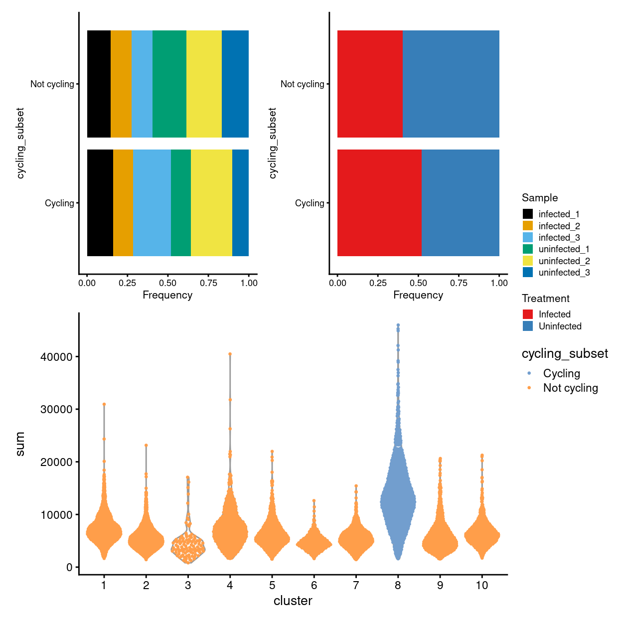
Cycling subset has larger library sizes
Show code
p3 <- plotColData(
  sce,
  "sum",
  x = "cluster",
  colour_by = "cycling_subset",
  point_size = 0.5,
  point_alpha = 1)
(p1 + p2) / p3 + plot_layout(guides = "collect")
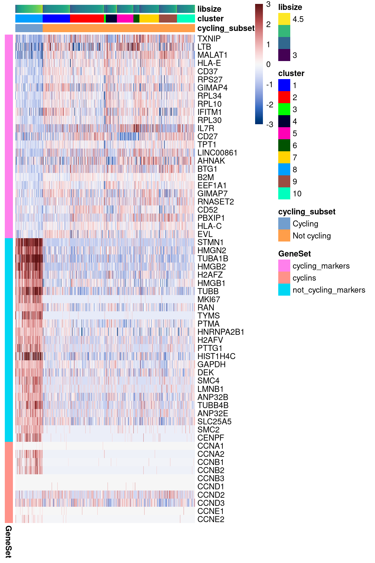
Expression of cycling subset markers and cyclins
Please see output/marker_genes/cycling_subset/ for heatmaps and spreadsheets of these marker gene lists.
Show code
cycling_subset_markers <- findMarkers(
  sce,
  sce$cycling_subset,
  direction = "up",
  block = sce$Sample,
  lfc = 0.5,
  row.data = flattenDF(rowData(sce)))

cyclin_genes <- grep("^CCN[ABDE][0-9]$", rowData(sce)$Symbol)
cyclin_genes <- sort(rownames(sce)[cyclin_genes])

features <- unlist(
  List(
    cycling_markers = head(
      rownames(cycling_subset_markers[["Not cycling"]]),
      25),
    not_cycling_markers = head(
      rownames(cycling_subset_markers[["Cycling"]]),
      25),
    cyclins = cyclin_genes))
plotHeatmap(
  sce,
  features,
  order_columns_by = c("cycling_subset", "cluster", "libsize"),
  cluster_rows = FALSE,
  color = hcl.colors(101, "Blue-Red 3"),
  center = TRUE,
  zlim = c(-3, 3),
  column_annotation_colors = list(cluster = cluster_colours),
  annotation_row = data.frame(
    GeneSet = names(features),
    row.names = features))
Show code
outdir <- here("output", "marker_genes", "cycling_subset")
dir.create(outdir, recursive = TRUE)
createClusterMarkerOutputs(
  sce = sce,
  outdir = outdir,
  markers = cycling_subset_markers,
  k = 100,
  width = 6,
  height = 7.5)
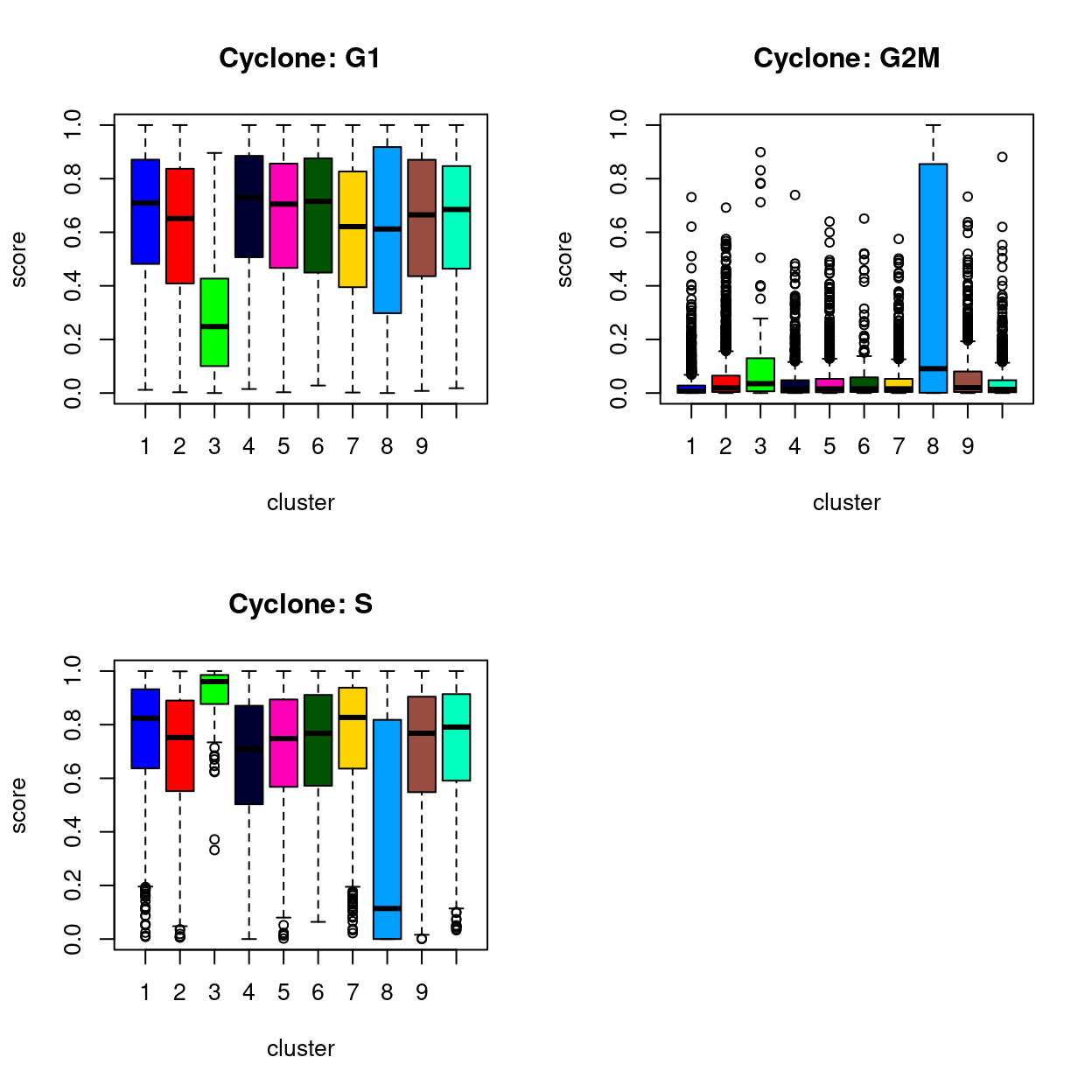
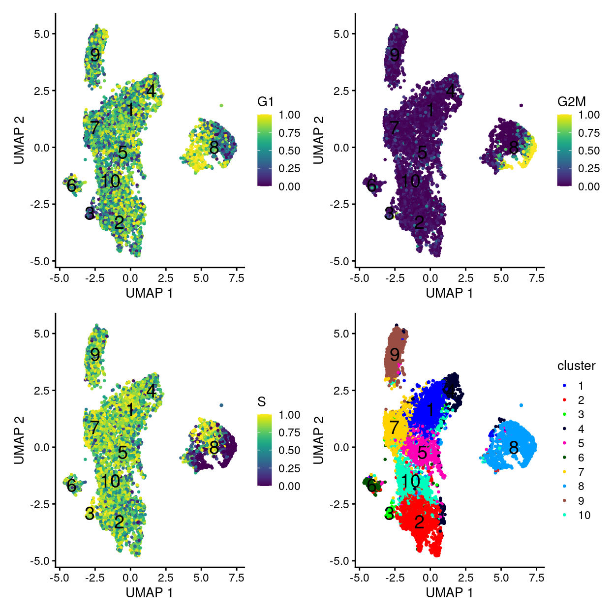
Using the cyclone() classifier
- Unsure how much I trust these results given the classifier was trained on quite a different dataset
Show code
# NOTE: This was run and the results saved.
# hs.pairs <- readRDS(system.file("exdata", "human_cycle_markers.rds",
#                                 package="scran"))
#
# # Using Ensembl IDs to match up with the annotation in 'hs.pairs'.
# set.seed(100)
# assignments <- cyclone(
#   sce,
#   hs.pairs,
#   gene.names = rowData(sce)$ENSEMBL.GENEID)
assignments <- readRDS(here("data", "cyclone_assignments.rds"))
colData(sce) <- cbind(colData(sce), DataFrame(assignments$score))
sce$phases <- assignments$phases
Show code
par(mfrow = c(2, 2))
boxplot(
  sce$G1 ~ sce$cluster,
  ylab = "score",
  col = cluster_colours,
  xlab = "cluster",
  main = "Cyclone: G1")
boxplot(
  sce$G2M ~ sce$cluster,
  ylab = "score",
  col = cluster_colours,
  xlab = "cluster",
  main = "Cyclone: G2M")
boxplot(
  sce$S ~ sce$cluster,
  ylab = "score",
  col = cluster_colours,
  xlab = "cluster",
  main = "Cyclone: S")
Show code
proportions(table(sce$cluster, assignments$phases), 1)
              G1         G2M           S
  1  0.738660907 0.002159827 0.259179266
  2  0.659289458 0.006988934 0.333721607
  3  0.163461538 0.057692308 0.778846154
  4  0.757246377 0.001811594 0.240942029
  5  0.726846424 0.003516999 0.269636577
  6  0.700657895 0.006578947 0.292763158
  7  0.647118301 0.001011122 0.351870576
  8  0.478136201 0.313978495 0.207885305
  9  0.698133919 0.006586169 0.295279912
  10 0.721919302 0.005452563 0.272628135
Show code
proportions(table(sce$cycling_subset, sce$phases), 1)
                       G1         G2M           S
  Cycling     0.478136201 0.313978495 0.207885305
  Not cycling 0.693381593 0.005041365 0.301577042
Show code
p1 <- plotUMAP(
  sce,
  colour_by = "G1",
  text_by = "cluster",
  point_size = 0.5,
  point_alpha = 1)
p2 <- plotUMAP(
  sce,
  colour_by = "G2M",
  text_by = "cluster",
  point_size = 0.5,
  point_alpha = 1)
p3 <- plotUMAP(
    sce,
    colour_by = "S",
    text_by = "cluster",
    point_size = 0.5,
    point_alpha = 1)
p4 <- plotUMAP(
    sce,
    colour_by = "cluster",
    text_by = "cluster",
    point_size = 0.5,
    point_alpha = 1) +
  scale_colour_manual(values = cluster_colours, name = "cluster")
p1 + p2 + p3 + p4 + plot_layout(ncol = 2)
Using the tricycle package
- tricycle (Transferable Representation and Inference of Cell Cycle) contains functions to infer and visualize cell cycle process using scRNA-seq data (Zheng et al. 2021)
Show code
library(tricycle)

# Project a single cell data set to pre-learned cell cycle space
sce <- project_cycle_space(
  x = sce,
  gname.type = "SYMBOL",
  species = "human")

# Diagnostic plot: should roughly be an ellipsoid (see
# http://bioconductor.org/packages/release/bioc/vignettes/tricycle/inst/doc/tricycle.html#assessing-performance)
# plotReducedDim(
#   sce,
#   dimred = "tricycleEmbedding",
#   point_alpha = 1) +
#   labs(x = "Projected PC1", y = "Projected PC2") +
#   ggtitle("Projected cell cycle space") +
#   theme_cowplot()
The main output of tricycle is a continuous estimate of the relative time within the cell cycle, represented as a number between \(0\) and \(2\pi\) (which we refer to as cell cycle position). According to the authors of tricycle:
We think the continuous position [rather than discrete stages] is more appropriate when describing the cell cycle. However, to help users understand the position variable, we also note that users can approximately relate:
- \(\pi/2\) to be the start of S stage
- \(\pi\) to be the start of G2M stage
- \(3\pi/2\) to be the middle of M stage
- \(7\pi/4 - \pi/4\) to be G1/G0 stage
Figure 1 shows the estimated cell cycle position of each cell. We observe that most cells have an estimated cell cycle position in \(7\pi/4 - \pi/4\) (i.e. consistent with G1/G0 stage) but that there is a cluster of cells with estimated cell cycle positions across the full range of values, i.e. cells in this cluster are going through various stages of the cell cycle.
Show code
# Infer cell cycle position
sce <- estimate_cycle_position(sce)

# Plot out embedding scater plot colored by cell cycle position
p <- plot_emb_circle_scale(
  sce,
  dimred = "UMAP",
  point.size = 1,
  point.alpha = 1,
  fig.title = "") +
  theme_cowplot()
legend <- circle_scale_legend(text.size = 4, alpha = 0.9)
plot_grid(p, legend, ncol = 2, rel_widths = c(1, 0.3))
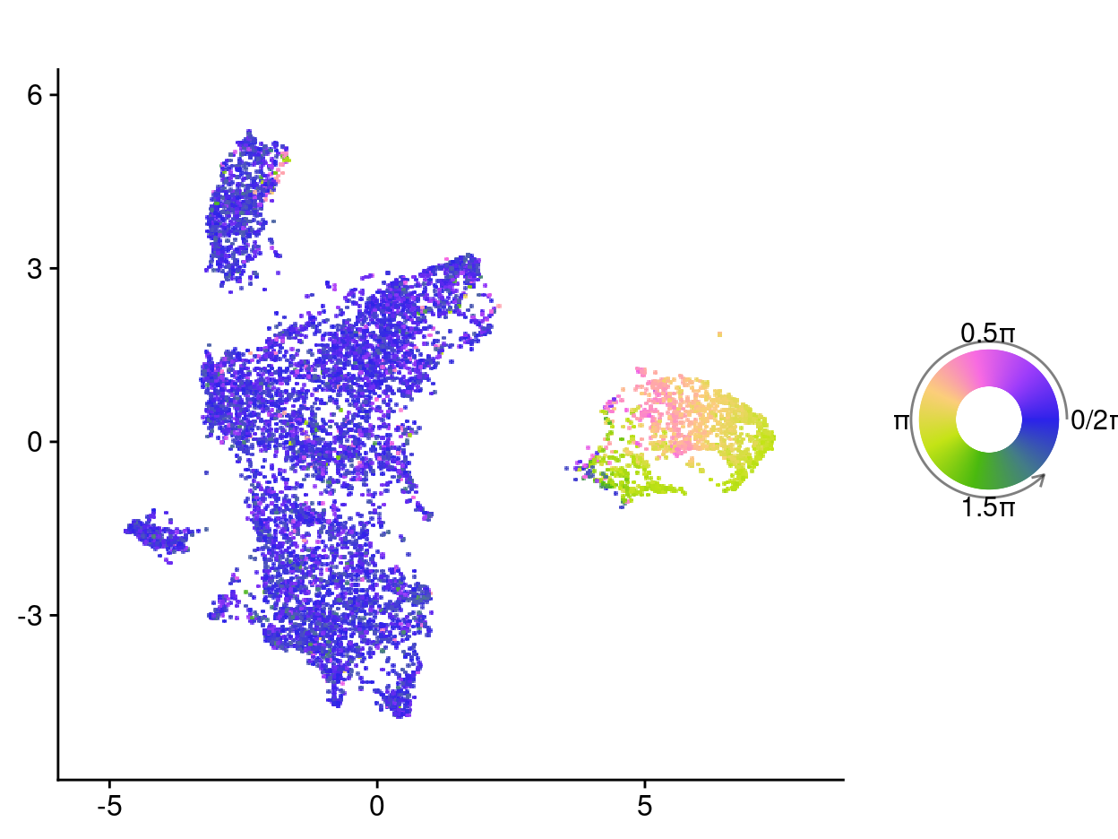
Figure 1: UMAP plot where each celll is coloured by its estimated cell cycle position. These values can be approximately related as follows: pi/2 to be the start of S stage; pi to be the start of G2M stage; 3pi/2 to be the middle of M stage; and 7pi/4 - pi/4 to be G1/G0 stage
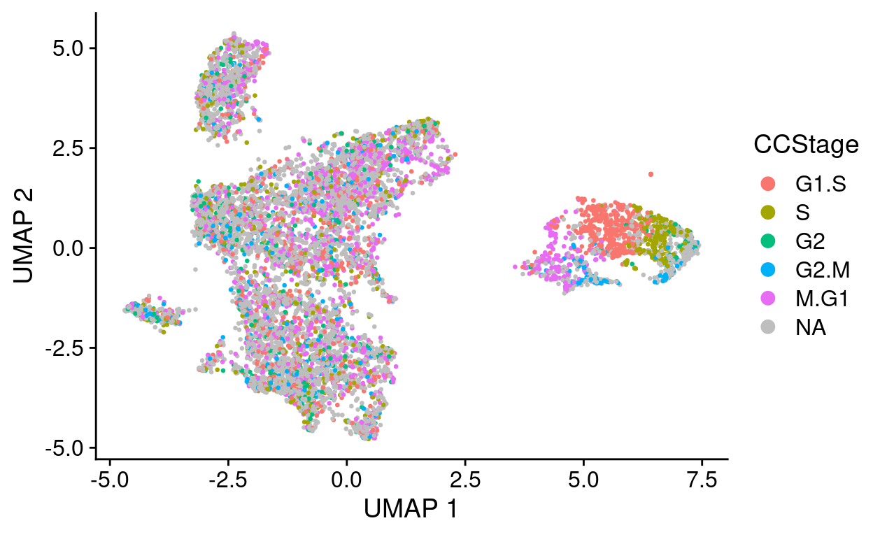
The authors of tricycle also offer a modified version of the Schwabe et al. (2020) cell cycle stage estimator.
Show code
# Alternative: Infer cell cycle stages
sce <- estimate_Schwabe_stage(
  x = sce,
  gname.type = "SYMBOL",
  species = "human")
Note that \(n =\) 4,865 cells (53%) cannot be assigned a cell stage by this procedure (CCStage is NA). Furthermore:
- Most of the cells in the main cluster are assigned a seemingly arbitrary stage, likely reflecting that these cells aren’t cycling and the algorithm cannot confidently assign these.
- The cells in the ‘cycling’ cluster are assigned clear, discrete cell stages that are consistent with preferred the estimated cell cycle values provided by tricycle.
Show code
plotUMAP(
  sce,
  colour_by = "CCStage",
  point_size = 0.5,
  point_alpha = 1) +
  theme_cowplot() +
  guides(colour = guide_legend(override.aes = list(size = 3))) +
  scale_colour_discrete(na.value = "grey", name = "CCStage")
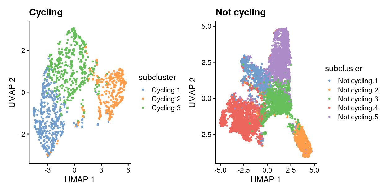
Subset analysis based on cycling_subset
- Using a fairly coarse clustering (
k = 50)
Show code
set.seed(9391)
list_of_sce <- quickSubCluster(
  sce,
  groups = sce$cycling_subset,
  prepFUN = function(x) {
    var_fit <- modelGeneVarByPoisson(x)
    hvg <- getTopHVGs(var_fit, var.threshold = 0)
    is_mito <- hvg %in% mito_set
    is_ribo <- hvg %in% ribo_set
    hvg <- hvg[!(is_mito | is_ribo)]
    # NOTE: Keep the original dimensionality reduction around for downstream
    #       plotting.
    reducedDimNames(x) <- paste0("original_", reducedDimNames(x))
    denoisePCA(x, var_fit, subset.row = hvg)
  },
  clusterFUN = function(x) {
    snn_gr <- buildSNNGraph(x, use.dimred = "PCA", k = 50)
    factor(igraph::cluster_louvain(snn_gr)$membership)
  })
# It's also useful to have per-sample UMAP representations.
set.seed(17127)
list_of_sce <- lapply(list_of_sce, runUMAP, dimred = "PCA")
Show code
# It's also useful to have SingleR DICE with fine labels for subclusters
library(SingleR)
library(celldex)
ref <- DatabaseImmuneCellExpressionData()
labels_fine <- ref$label.fine
# NOTE: This code doesn't necessarily generalise beyond the DICE main labels.
label_fine_collapsed_colours <- setNames(
  c(
    Polychrome::glasbey.colors(nlevels(factor(labels_fine)) + 1)[-1],
    "orange"),
  c(levels(factor(labels_fine)), "other"))
list_of_sce <- lapply(list_of_sce, function(x) {
  pred_subcluster_fine <- SingleR(
    test = x,
    ref = ref,
    labels = labels_fine,
    clusters = x$subcluster)
  x$label_subcluster_fine <- factor(
    pred_subcluster_fine[x$subcluster, "pruned.labels"])
  x
})
list_of_sce <- lapply(list_of_sce, function(x) {
  pred_cell_fine <- SingleR(
    test = x,
    ref = ref,
    labels = labels_fine)
  x$label_cell_fine <- factor(pred_cell_fine$pruned.labels)
  x
})
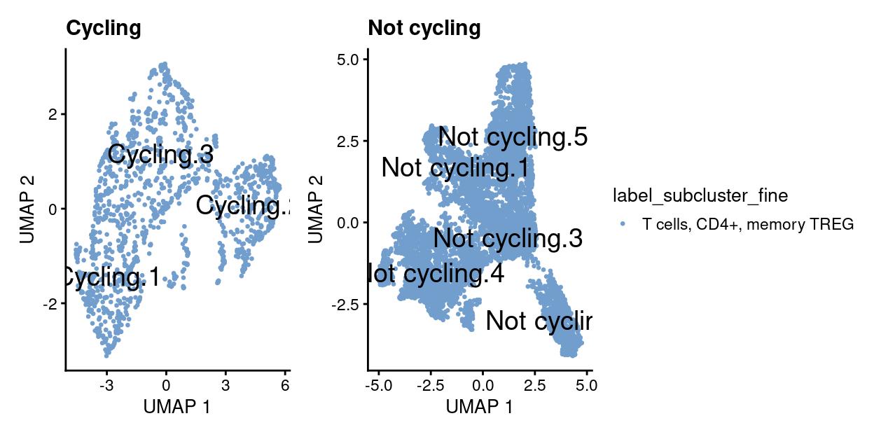
Show code
wrap_plots(
  lapply(names(list_of_sce), function(n) {
    x <- list_of_sce[[n]]
    plotUMAP(x, colour_by = "subcluster", point_size = 0.5, point_alpha = 1) +
      ggtitle(n)
  }))
Show code
wrap_plots(
  lapply(names(list_of_sce), function(n) {
    x <- list_of_sce[[n]]
    plotUMAP(
      x,
      colour_by = "label_subcluster_fine",
      text_by = "subcluster",
      point_size = 0.5,
      point_alpha = 1) +
      ggtitle(n)
  })) +
  plot_layout(guides = "collect")
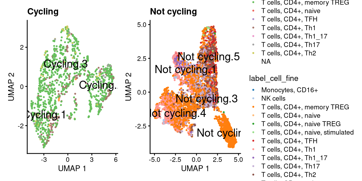
Show code
wrap_plots(
  lapply(names(list_of_sce), function(n) {
    x <- list_of_sce[[n]]
    plotUMAP(
      x,
      colour_by = "label_cell_fine",
      text_by = "subcluster",
      point_size = 0.5,
      point_alpha = 1) +
      ggtitle(n)
  })) +
  plot_layout(guides = "collect")
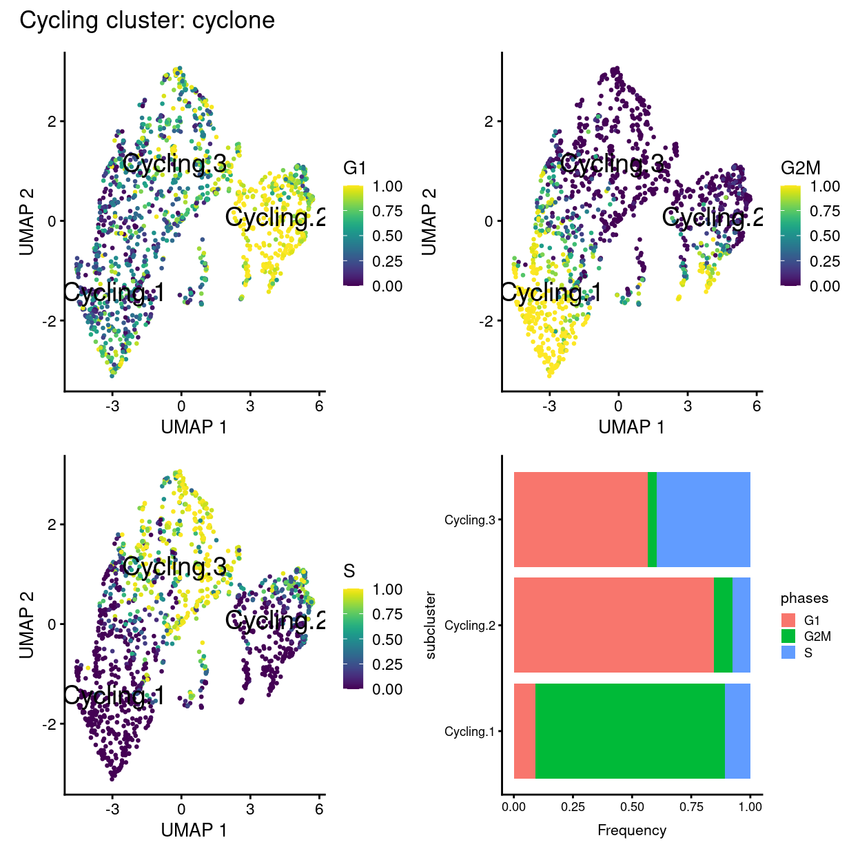
Cycling subset analysis
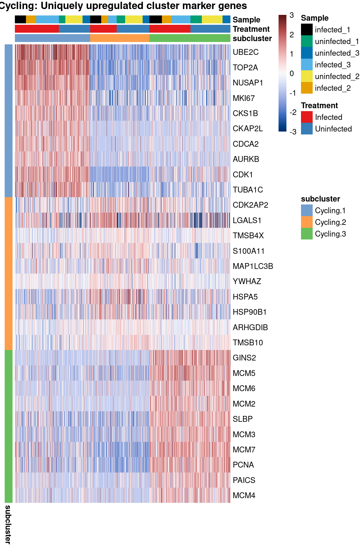
Please see output/marker_genes/cycling_subset_subclusters/ for heatmaps and spreadsheets of these marker gene lists.
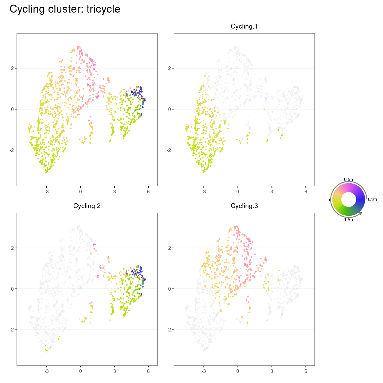
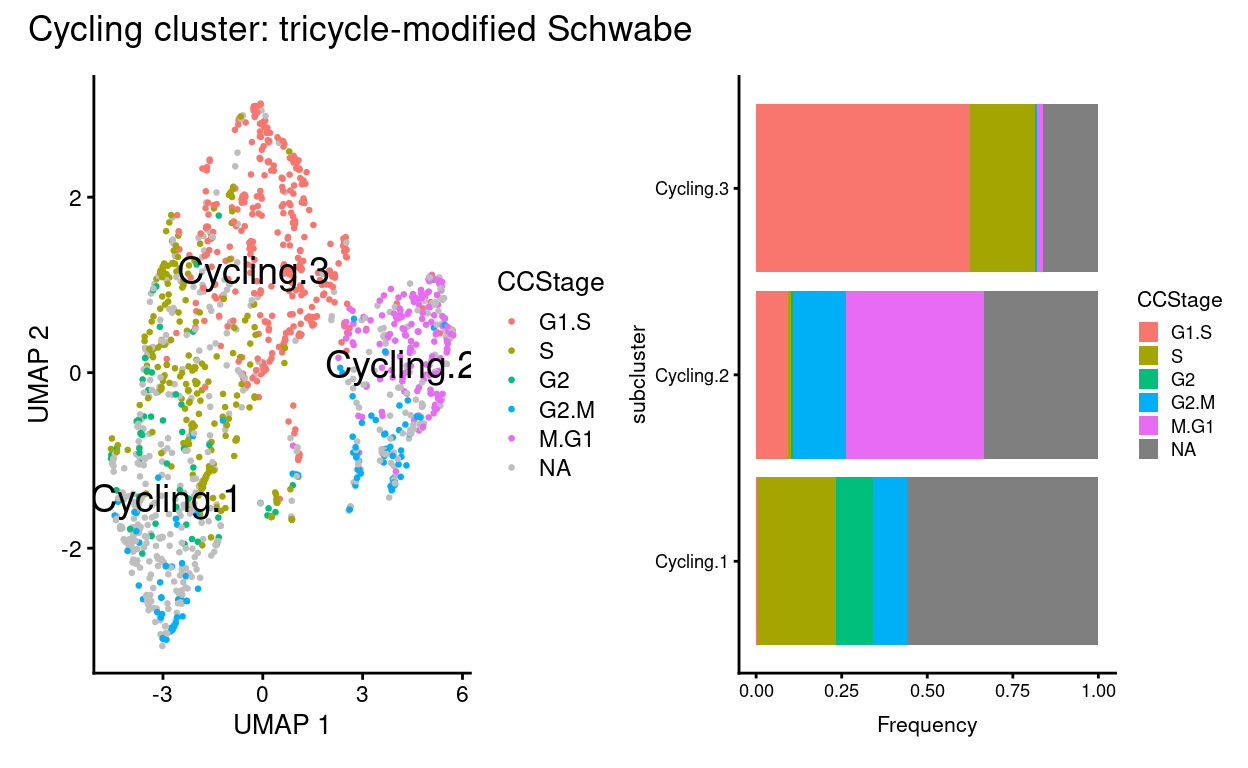
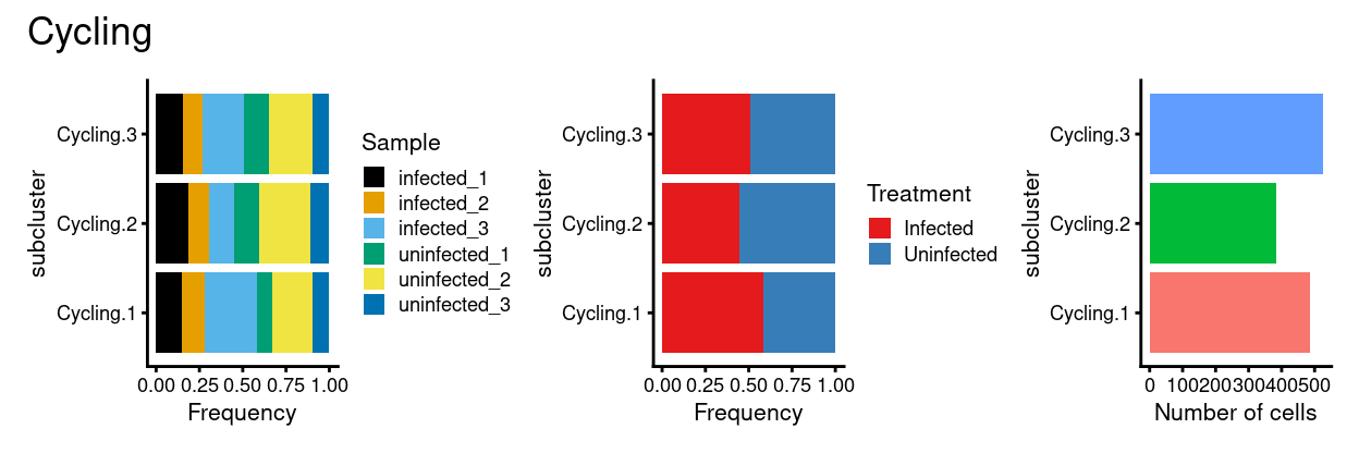
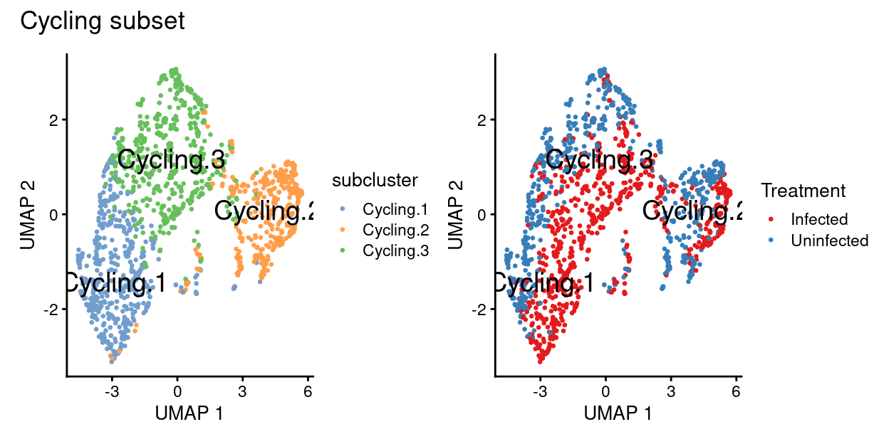
Cyclingsubset subclusters are strongly enriched for cyclone’s predicted cell cycle phase (phases), tricycle’s estimated cell cycle position, and tricycle-modified Schwabe cell stages (CCStage).Cyclingsubset subclusters have strong marker genes (but these probably reflect more cell cycle and less cell type)Cyclingsubset subclusters don’t appear to beTreatment-specific
Show code
cycling_sce <- list_of_sce[["Cycling"]]
colLabels(cycling_sce) <- cycling_sce$subcluster
Show code
wrap_plots(
  plotlist = c(
    lapply(c("G1", "G2M", "S"), function(phase) {
      plotUMAP(
        cycling_sce,
        colour_by = phase,
        text_by = "subcluster",
        point_size = 0.5,
        point_alpha = 1)
    }),
    list(
      ggplot(
        as.data.frame(
          colData(cycling_sce)[, c("subcluster", "phases")])) +
        geom_bar(
          aes(x = subcluster, fill = phases),
          position = position_fill(reverse = TRUE)) +
        coord_flip() +
        ylab("Frequency") +
        theme_cowplot(font_size = 8)))) +
  plot_annotation(title = "Cycling cluster: cyclone")
Show code
(wrap_plots(
  plot_emb_circle_scale(
    cycling_sce,
    dimred = "UMAP",
    point.size = 2,
    point.alpha = 1,
    fig.title = "",
    facet_by = "subcluster")) |
   circle_scale_legend(text.size = 2, alpha = 0.9)) +
  plot_layout(widths = c(1, 0.2)) +
  plot_annotation(title = "Cycling cluster: tricycle")
Show code
wrap_plots(
  plotlist = c(
    list(
      plotUMAP(
      cycling_sce,
      colour_by = "CCStage",
      text_by = "subcluster",
      point_size = 0.5,
      point_alpha = 1) +
        scale_colour_discrete(na.value = "grey", name = "CCStage")
    ),
    list(
      ggplot(
        as.data.frame(
          colData(cycling_sce)[, c("subcluster", "CCStage")])) +
        geom_bar(
          aes(x = subcluster, fill = CCStage),
          position = position_fill(reverse = TRUE)) +
        coord_flip() +
        ylab("Frequency") +
        theme_cowplot(font_size = 8)))) +
  plot_annotation(title = "Cycling cluster: tricycle-modified Schwabe")
Show code
out <- pairwiseTTests(
  cycling_sce,
  cycling_sce$subcluster,
  direction = "up",
  block = cycling_sce$Sample)
top_markers <- getTopMarkers(
  out$statistics,
  out$pairs,
  pairwise = FALSE,
  pval.type = "all",
  n = 10)
features <- unlist(top_markers)
plotHeatmap(
  cycling_sce,
  features,
  order_columns_by = c("subcluster", "Treatment", "Sample"),
  cluster_rows = FALSE,
  color = hcl.colors(101, "Blue-Red 3"),
  center = TRUE,
  zlim = c(-3, 3),
  column_annotation_colors = list(
    Treatment = treatment_colours,
    Sample = sample_colours),
  annotation_row = data.frame(
    subcluster = names(features),
    row.names = features),
  main = "Cycling: Uniquely upregulated cluster marker genes")
Show code
p1 <- ggplot(as.data.frame(colData(cycling_sce)[, c("subcluster", "Sample")])) +
    geom_bar(
      aes(x = subcluster, fill = Sample),
      position = position_fill(reverse = TRUE)) +
    coord_flip() +
    ylab("Frequency") +
    scale_fill_manual(values = sample_colours) +
    theme_cowplot(font_size = 8)
p2 <- ggplot(as.data.frame(colData(cycling_sce)[, c("subcluster", "Treatment")])) +
    geom_bar(
      aes(x = subcluster, fill = Treatment),
      position = position_fill(reverse = TRUE)) +
    coord_flip() +
    ylab("Frequency") +
    scale_fill_manual(values = treatment_colours) +
    theme_cowplot(font_size = 8)
p3 <- ggplot(as.data.frame(colData(cycling_sce)[, "subcluster", drop = FALSE])) +
    geom_bar(aes(x = subcluster, fill = subcluster)) +
    coord_flip() +
    ylab("Number of cells") +
    theme_cowplot(font_size = 8) +
    guides(fill = FALSE)

p1 + p2 + p3 + plot_annotation(title = "Cycling")
Show code
p1 <- plotUMAP(
  cycling_sce,
  colour_by = "subcluster",
  text_by = "subcluster",
  point_size = 0.5,
  point_alpha = 1)
p2 <- plotUMAP(
  cycling_sce,
  colour_by = "Treatment",
  text_by = "subcluster",
  point_size = 0.5,
  point_alpha = 1) +
  scale_colour_manual(values = treatment_colours, name = "Treatment")
p1 + p2 + plot_annotation("Cycling subset")
Show code
markers <- findMarkers(
  cycling_sce,
  cycling_sce$subcluster,
  direction = "up",
  pval.type = "all",
  block = cycling_sce$Sample,
  row.data = flattenDF(rowData(cycling_sce)))
outdir <- here("output", "marker_genes", "cycling_subset_subcluster")
dir.create(outdir, recursive = TRUE)
createClusterMarkerOutputs(
  sce = cycling_sce,
  outdir = outdir,
  markers = markers,
  k = 100,
  width = 6,
  height = 7.5)
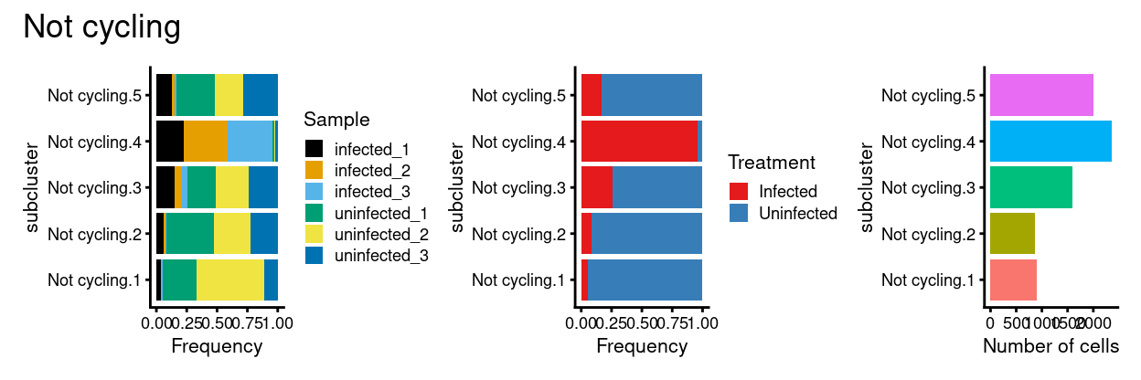
Not cycling subset analysis
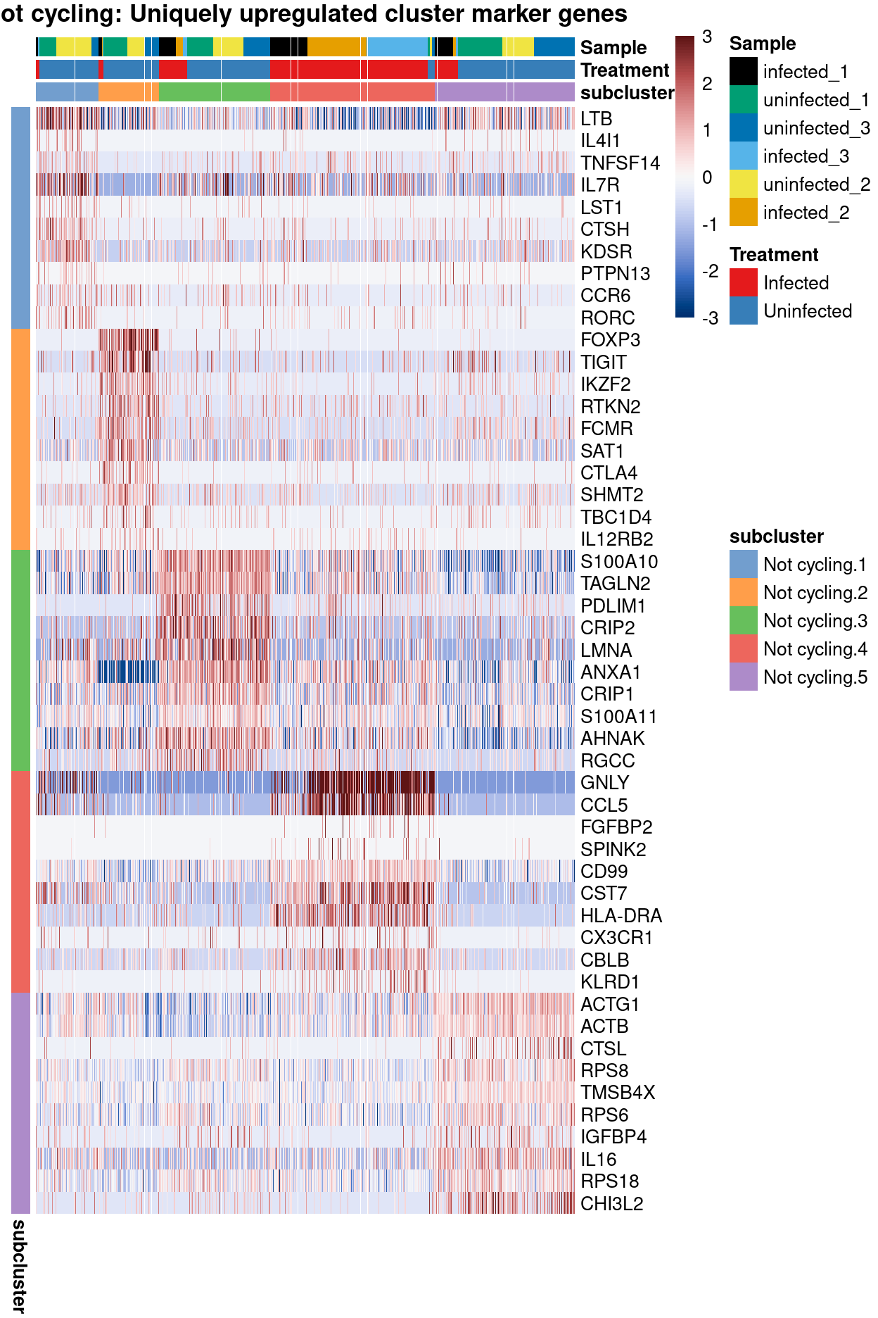
Please see output/marker_genes/not_cycling_subset_subclusters/ for heatmaps and spreadsheets of these marker gene lists.
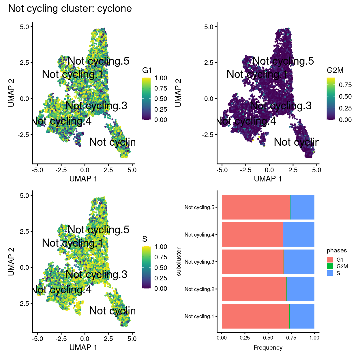
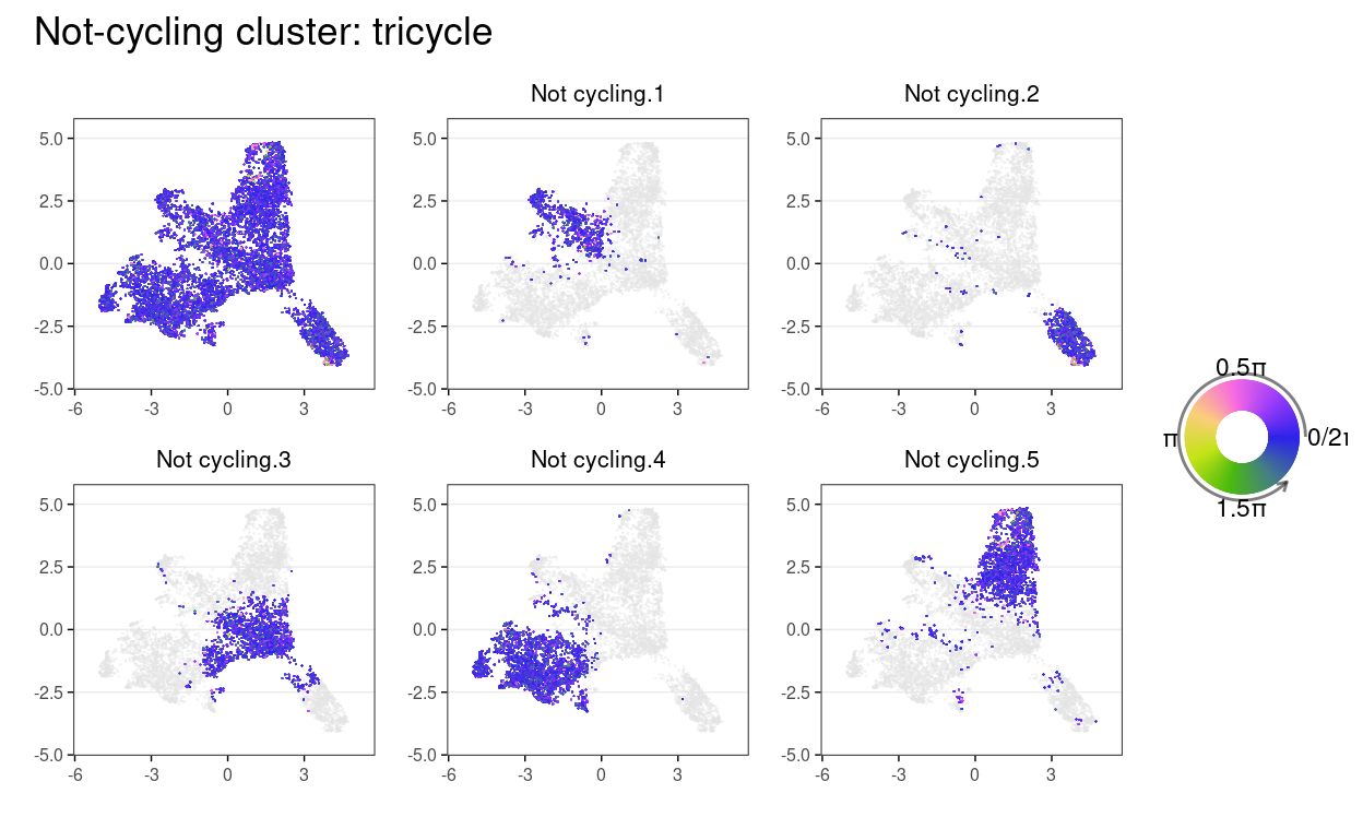
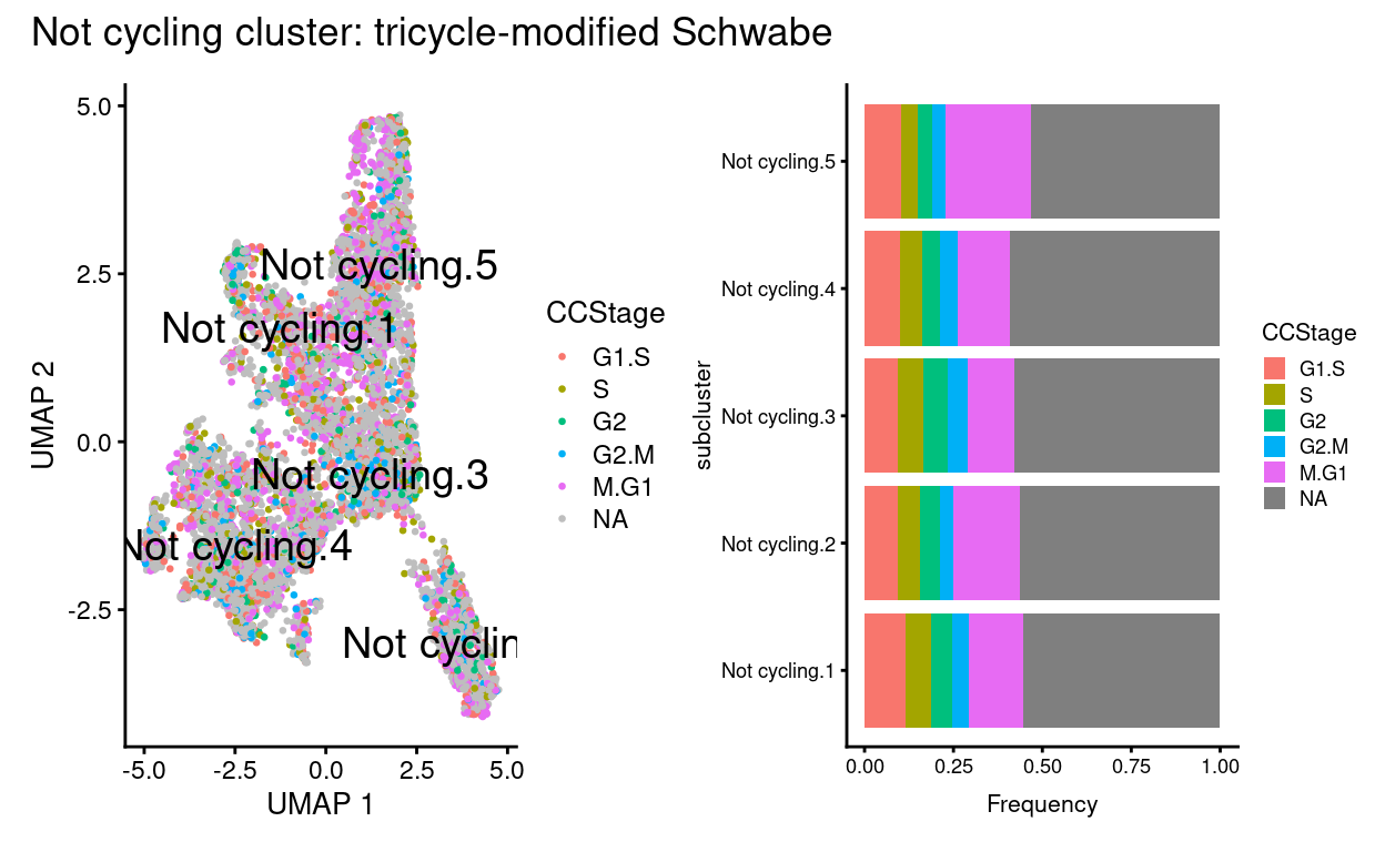
Not cyclingsubset subclusters have little association with cyclone’s predicted cell cycle phase (phases), tricycle’s estimated cell cycle position, or tricycle-modified Schwabe cell stages (CCStage).- This is kind of obvious because by definition these cells aren’t thought to be cycling!
Not cyclingsubset subclusters have strong marker genes (likely reflecting cell type / state)Not cyclingsubset subclusters appear to be highlyTreatment-specific
Show code
not_cycling_sce <- list_of_sce[["Not cycling"]]
colLabels(not_cycling_sce) <- not_cycling_sce$subcluster
Show code
wrap_plots(
  plotlist = c(
    lapply(c("G1", "G2M", "S"), function(phase) {
      plotUMAP(
        not_cycling_sce,
        colour_by = phase,
        text_by = "subcluster",
        point_size = 0.5,
        point_alpha = 1)
    }),
    list(
      ggplot(
        as.data.frame(
          colData(not_cycling_sce)[, c("subcluster", "phases")])) +
        geom_bar(
          aes(x = subcluster, fill = phases),
          position = position_fill(reverse = TRUE)) +
        coord_flip() +
        ylab("Frequency") +
        theme_cowplot(font_size = 8)))) +
  plot_annotation(title = "Not cycling cluster: cyclone")
Show code
(wrap_plots(
  plot_emb_circle_scale(
    not_cycling_sce,
    dimred = "UMAP",
    point.size = 2,
    point.alpha = 1,
    fig.title = "",
    facet_by = "subcluster")) |
   circle_scale_legend(text.size = 3, alpha = 0.9)) +
  plot_layout(widths = c(1, 0.2)) +
  plot_annotation(title = "Not-cycling cluster: tricycle")
Show code
wrap_plots(
  plotlist = c(
    list(
      plotUMAP(
      not_cycling_sce,
      colour_by = "CCStage",
      text_by = "subcluster",
      point_size = 0.5,
      point_alpha = 1) +
        scale_colour_discrete(na.value = "grey", name = "CCStage")
    ),
    list(
      ggplot(
        as.data.frame(
          colData(not_cycling_sce)[, c("subcluster", "CCStage")])) +
        geom_bar(
          aes(x = subcluster, fill = CCStage),
          position = position_fill(reverse = TRUE)) +
        coord_flip() +
        ylab("Frequency") +
        theme_cowplot(font_size = 8)))) +
  plot_annotation(title = "Not cycling cluster: tricycle-modified Schwabe")
Show code
out <- pairwiseTTests(
  not_cycling_sce,
  not_cycling_sce$subcluster,
  direction = "up",
  block = not_cycling_sce$Sample)
top_markers <- getTopMarkers(
  out$statistics,
  out$pairs,
  pairwise = FALSE,
  pval.type = "all",
  n = 10)
features <- unlist(top_markers)
plotHeatmap(
  not_cycling_sce,
  features,
  order_columns_by = c("subcluster", "Treatment", "Sample"),
  cluster_rows = FALSE,
  color = hcl.colors(101, "Blue-Red 3"),
  center = TRUE,
  zlim = c(-3, 3),
  column_annotation_colors = list(
    Treatment = treatment_colours,
    Sample = sample_colours),
  annotation_row = data.frame(
    subcluster = names(features),
    row.names = features),
  main = "Not cycling: Uniquely upregulated cluster marker genes")
Show code
p1 <- ggplot(
  as.data.frame(colData(not_cycling_sce)[, c("subcluster", "Sample")])) +
    geom_bar(
      aes(x = subcluster, fill = Sample),
      position = position_fill(reverse = TRUE)) +
    coord_flip() +
    ylab("Frequency") +
    scale_fill_manual(values = sample_colours) +
    theme_cowplot(font_size = 8)
p2 <- ggplot(
  as.data.frame(colData(not_cycling_sce)[, c("subcluster", "Treatment")])) +
    geom_bar(
      aes(x = subcluster, fill = Treatment),
      position = position_fill(reverse = TRUE)) +
    coord_flip() +
    ylab("Frequency") +
    scale_fill_manual(values = treatment_colours) +
    theme_cowplot(font_size = 8)
p3 <- ggplot(
  as.data.frame(colData(not_cycling_sce)[, "subcluster", drop = FALSE])) +
    geom_bar(aes(x = subcluster, fill = subcluster)) +
    coord_flip() +
    ylab("Number of cells") +
    theme_cowplot(font_size = 8) +
    guides(fill = FALSE)

p1 + p2 + p3 + plot_annotation(title = "Not cycling")
Show code
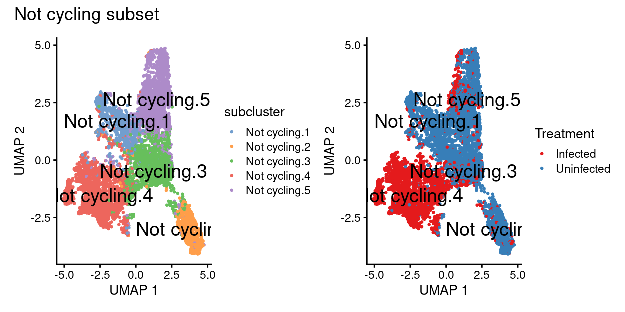
p1 <- plotUMAP(
  not_cycling_sce,
  colour_by = "subcluster",
  text_by = "subcluster",
  point_size = 0.5,
  point_alpha = 1)
p2 <- plotUMAP(
  not_cycling_sce,
  colour_by = "Treatment",
  text_by = "subcluster",
  point_size = 0.5,
  point_alpha = 1) +
  scale_colour_manual(values = treatment_colours, name = "Treatment")
p1 + p2 + plot_annotation("Not cycling subset")
Show code
markers <- findMarkers(
  not_cycling_sce,
  not_cycling_sce$subcluster,
  direction = "up",
  pval.type = "all",
  block = not_cycling_sce$Sample,
  row.data = flattenDF(rowData(not_cycling_sce)))
outdir <- here("output", "marker_genes", "not_cycling_subset_subcluster")
dir.create(outdir, recursive = TRUE)
createClusterMarkerOutputs(
  sce = not_cycling_sce,
  outdir = outdir,
  markers = markers,
  k = 100,
  width = 6,
  height = 7.5)
Concluding remarks
Show code
The processed SingleCellExperiment objects are available (see data/SCEs/C057_Cooney.cells_selected.SCE.rds, data/SCEs/C057_Cooney.cycling.annotated.SCE.rds, and data/SCEs/C057_Cooney.not_cycling.annotated.SCE.rds). These will be used in downstream analyses, e.g., differential expression analysis between conditions within each cluster and differential abundance analyses between conditions for each cluster.
Additional information
The following are available on request:
- Full CSV tables of any data presented.
- PDF/PNG files of any static plots.
Session info
Show code
sessioninfo::session_info()
─ Session info ─────────────────────────────────────────────────────
 setting  value
 version  R version 4.0.3 (2020-10-10)
 os       CentOS Linux 7 (Core)
 system   x86_64, linux-gnu
 ui       X11
 language (EN)
 collate  en_US.UTF-8
 ctype    en_US.UTF-8
 tz       Australia/Melbourne
 date     2021-07-01

─ Packages ─────────────────────────────────────────────────────────
 ! package                * version  date       lib
 P AnnotationDbi            1.52.0   2020-10-27 [?]
 P AnnotationHub            2.22.0   2020-10-27 [?]
 P assertthat               0.2.1    2019-03-21 [?]
 P batchelor              * 1.6.2    2020-11-26 [?]
 P beachmat                 2.6.4    2020-12-20 [?]
 P beeswarm                 0.2.3    2016-04-25 [?]
 P Biobase                * 2.50.0   2020-10-27 [?]
   BiocFileCache            1.14.0   2020-10-27 [1]
   BiocGenerics           * 0.36.0   2020-10-27 [1]
 P BiocManager              1.30.10  2019-11-16 [?]
 P BiocNeighbors            1.8.2    2020-12-07 [?]
   BiocParallel             1.24.1   2020-11-06 [1]
 P BiocSingular             1.6.0    2020-10-27 [?]
   BiocStyle                2.18.1   2020-11-24 [1]
   BiocVersion              3.12.0   2020-04-27 [1]
 P bit                      4.0.4    2020-08-04 [?]
 P bit64                    4.0.5    2020-08-30 [?]
 P bitops                   1.0-6    2013-08-17 [?]
 P blob                     1.2.1    2020-01-20 [?]
 P bluster                  1.0.0    2020-10-27 [?]
 P boot                     1.3-27   2021-02-12 [?]
 P bslib                    0.2.4    2021-01-25 [?]
 P cachem                   1.0.4    2021-02-13 [?]
 P celldex                * 1.0.0    2020-10-29 [?]
 P circular                 0.4-93   2017-06-29 [?]
 P cli                      2.3.1    2021-02-23 [?]
 P codetools                0.2-18   2020-11-04 [?]
 P colorspace               2.0-0    2020-11-11 [?]
 P cowplot                * 1.1.1    2020-12-30 [?]
 P crayon                   1.4.1    2021-02-08 [?]
 P crosstalk                1.1.1    2021-01-12 [?]
 P curl                     4.3      2019-12-02 [?]
 P DBI                      1.1.1    2021-01-15 [?]
 P dbplyr                   2.1.0    2021-02-03 [?]
 P DelayedArray             0.16.2   2021-02-26 [?]
 P DelayedMatrixStats       1.12.3   2021-02-03 [?]
 P digest                   0.6.27   2020-10-24 [?]
 P distill                  1.2      2021-01-13 [?]
 P downlit                  0.2.1    2020-11-04 [?]
 P dplyr                    1.0.4    2021-02-02 [?]
 P dqrng                    0.2.1    2019-05-17 [?]
 P DT                       0.17     2021-01-06 [?]
 P edgeR                    3.32.1   2021-01-14 [?]
 P ellipsis                 0.3.1    2020-05-15 [?]
 P evaluate                 0.14     2019-05-28 [?]
 P ExperimentHub            1.16.0   2020-10-27 [?]
 P fansi                    0.4.2    2021-01-15 [?]
 P farver                   2.1.0    2021-02-28 [?]
 P fastmap                  1.1.0    2021-01-25 [?]
 P FNN                      1.1.3    2019-02-15 [?]
 P generics                 0.1.0    2020-10-31 [?]
 P GenomeInfoDb           * 1.26.2   2020-12-08 [?]
   GenomeInfoDbData         1.2.4    2021-02-04 [1]
 P GenomicRanges          * 1.42.0   2020-10-27 [?]
 P ggbeeswarm               0.6.0    2017-08-07 [?]
 P ggplot2                * 3.3.3    2020-12-30 [?]
 P glue                     1.4.2    2020-08-27 [?]
 P GO.db                    3.12.1   2020-11-04 [?]
 P gridExtra                2.3      2017-09-09 [?]
 P gtable                   0.3.0    2019-03-25 [?]
 P here                   * 1.0.1    2020-12-13 [?]
 P highr                    0.8      2019-03-20 [?]
 P htmltools                0.5.1.1  2021-01-22 [?]
 P htmlwidgets              1.5.3    2020-12-10 [?]
 P httpuv                   1.5.5    2021-01-13 [?]
 P httr                     1.4.2    2020-07-20 [?]
 P igraph                   1.2.6    2020-10-06 [?]
 P interactiveDisplayBase   1.28.0   2020-10-27 [?]
 P IRanges                * 2.24.1   2020-12-12 [?]
 P irlba                    2.3.3    2019-02-05 [?]
 P jquerylib                0.1.3    2020-12-17 [?]
 P jsonlite                 1.7.2    2020-12-09 [?]
 P knitr                    1.31     2021-01-27 [?]
 P labeling                 0.4.2    2020-10-20 [?]
 P later                    1.1.0.1  2020-06-05 [?]
 P lattice                  0.20-41  2020-04-02 [?]
 P lifecycle                1.0.0    2021-02-15 [?]
   limma                  * 3.46.0   2020-10-27 [1]
 P locfit                   1.5-9.4  2020-03-25 [?]
 P magrittr               * 2.0.1    2020-11-17 [?]
 P Matrix                   1.3-2    2021-01-06 [?]
   MatrixGenerics         * 1.2.1    2021-01-30 [1]
 P matrixStats            * 0.58.0   2021-01-29 [?]
 P memoise                  2.0.0    2021-01-26 [?]
 P mime                     0.10     2021-02-13 [?]
 P msigdbr                * 7.2.1    2020-10-02 [?]
 P munsell                  0.5.0    2018-06-12 [?]
 P mvtnorm                  1.1-2    2021-06-07 [?]
 P org.Hs.eg.db             3.12.0   2020-10-20 [?]
 P patchwork              * 1.1.1    2020-12-17 [?]
 P pheatmap                 1.0.12   2019-01-04 [?]
 P pillar                   1.5.0    2021-02-22 [?]
 P pkgconfig                2.0.3    2019-09-22 [?]
 P Polychrome               1.2.6    2020-11-11 [?]
 P promises                 1.2.0.1  2021-02-11 [?]
 P purrr                    0.3.4    2020-04-17 [?]
 P R6                       2.5.0    2020-10-28 [?]
 P rappdirs                 0.3.3    2021-01-31 [?]
 P RColorBrewer             1.1-2    2014-12-07 [?]
 P Rcpp                     1.0.6    2021-01-15 [?]
 P RcppAnnoy                0.0.18   2020-12-15 [?]
 P RCurl                    1.98-1.2 2020-04-18 [?]
 P ResidualMatrix           1.0.0    2020-10-27 [?]
 P rlang                    0.4.10   2020-12-30 [?]
 P rmarkdown                2.7      2021-02-19 [?]
 P rprojroot                2.0.2    2020-11-15 [?]
 P RSpectra                 0.16-0   2019-12-01 [?]
 P RSQLite                  2.2.3    2021-01-24 [?]
 P rsvd                     1.0.3    2020-02-17 [?]
 P S4Vectors              * 0.28.1   2020-12-09 [?]
 P sass                     0.3.1    2021-01-24 [?]
 P scales                   1.1.1    2020-05-11 [?]
 P scater                 * 1.18.6   2021-02-26 [?]
 P scattermore              0.7      2020-11-24 [?]
 P scatterplot3d            0.3-41   2018-03-14 [?]
 P scran                  * 1.18.5   2021-02-04 [?]
 P scuttle                  1.0.4    2020-12-17 [?]
 P sessioninfo              1.1.1    2018-11-05 [?]
 P shiny                    1.6.0    2021-01-25 [?]
 P SingleCellExperiment   * 1.12.0   2020-10-27 [?]
 P SingleR                * 1.4.1    2021-02-02 [?]
 P sparseMatrixStats        1.2.1    2021-02-02 [?]
 P statmod                  1.4.35   2020-10-19 [?]
 P stringi                  1.5.3    2020-09-09 [?]
 P stringr                  1.4.0    2019-02-10 [?]
 P SummarizedExperiment   * 1.20.0   2020-10-27 [?]
 P tibble                   3.1.0    2021-02-25 [?]
 P tidyselect               1.1.0    2020-05-11 [?]
 P tricycle               * 0.99.32  2021-05-19 [?]
 P utf8                     1.1.4    2018-05-24 [?]
 P uwot                     0.1.10   2020-12-15 [?]
 P vctrs                    0.3.6    2020-12-17 [?]
 P vipor                    0.4.5    2017-03-22 [?]
 P viridis                  0.5.1    2018-03-29 [?]
 P viridisLite              0.3.0    2018-02-01 [?]
 P withr                    2.4.1    2021-01-26 [?]
 P xfun                     0.21     2021-02-10 [?]
 P xtable                   1.8-4    2019-04-21 [?]
 P XVector                  0.30.0   2020-10-27 [?]
 P yaml                     2.2.1    2020-02-01 [?]
 P zlibbioc                 1.36.0   2020-10-27 [?]
 source
 Bioconductor
 Bioconductor
 CRAN (R 4.0.0)
 Bioconductor
 Bioconductor
 CRAN (R 4.0.0)
 Bioconductor
 Bioconductor
 Bioconductor
 CRAN (R 4.0.0)
 Bioconductor
 Bioconductor
 Bioconductor
 Bioconductor
 Bioconductor
 CRAN (R 4.0.0)
 CRAN (R 4.0.0)
 CRAN (R 4.0.0)
 CRAN (R 4.0.0)
 Bioconductor
 CRAN (R 4.0.3)
 CRAN (R 4.0.3)
 CRAN (R 4.0.3)
 Bioconductor
 CRAN (R 4.0.3)
 CRAN (R 4.0.3)
 CRAN (R 4.0.3)
 CRAN (R 4.0.3)
 CRAN (R 4.0.3)
 CRAN (R 4.0.3)
 CRAN (R 4.0.3)
 CRAN (R 4.0.0)
 CRAN (R 4.0.3)
 CRAN (R 4.0.3)
 Bioconductor
 Bioconductor
 CRAN (R 4.0.2)
 CRAN (R 4.0.3)
 CRAN (R 4.0.3)
 CRAN (R 4.0.3)
 CRAN (R 4.0.0)
 CRAN (R 4.0.3)
 Bioconductor
 CRAN (R 4.0.0)
 CRAN (R 4.0.0)
 Bioconductor
 CRAN (R 4.0.3)
 CRAN (R 4.0.3)
 CRAN (R 4.0.3)
 CRAN (R 4.0.0)
 CRAN (R 4.0.3)
 Bioconductor
 Bioconductor
 Bioconductor
 CRAN (R 4.0.0)
 CRAN (R 4.0.3)
 CRAN (R 4.0.0)
 Bioconductor
 CRAN (R 4.0.0)
 CRAN (R 4.0.0)
 CRAN (R 4.0.3)
 CRAN (R 4.0.0)
 CRAN (R 4.0.3)
 CRAN (R 4.0.3)
 CRAN (R 4.0.3)
 CRAN (R 4.0.0)
 CRAN (R 4.0.2)
 Bioconductor
 Bioconductor
 CRAN (R 4.0.0)
 CRAN (R 4.0.3)
 CRAN (R 4.0.3)
 CRAN (R 4.0.3)
 CRAN (R 4.0.0)
 CRAN (R 4.0.0)
 CRAN (R 4.0.0)
 CRAN (R 4.0.3)
 Bioconductor
 CRAN (R 4.0.0)
 CRAN (R 4.0.3)
 CRAN (R 4.0.3)
 Bioconductor
 CRAN (R 4.0.3)
 CRAN (R 4.0.3)
 CRAN (R 4.0.3)
 CRAN (R 4.0.2)
 CRAN (R 4.0.0)
 CRAN (R 4.0.3)
 Bioconductor
 CRAN (R 4.0.3)
 CRAN (R 4.0.0)
 CRAN (R 4.0.3)
 CRAN (R 4.0.0)
 CRAN (R 4.0.3)
 CRAN (R 4.0.3)
 CRAN (R 4.0.0)
 CRAN (R 4.0.2)
 CRAN (R 4.0.3)
 CRAN (R 4.0.0)
 CRAN (R 4.0.3)
 CRAN (R 4.0.3)
 CRAN (R 4.0.0)
 Bioconductor
 CRAN (R 4.0.3)
 CRAN (R 4.0.3)
 CRAN (R 4.0.3)
 CRAN (R 4.0.0)
 CRAN (R 4.0.3)
 CRAN (R 4.0.0)
 Bioconductor
 CRAN (R 4.0.3)
 CRAN (R 4.0.0)
 Bioconductor
 CRAN (R 4.0.3)
 CRAN (R 4.0.0)
 Bioconductor
 Bioconductor
 CRAN (R 4.0.0)
 CRAN (R 4.0.3)
 Bioconductor
 Bioconductor
 Bioconductor
 CRAN (R 4.0.2)
 CRAN (R 4.0.0)
 CRAN (R 4.0.0)
 Bioconductor
 CRAN (R 4.0.3)
 CRAN (R 4.0.0)
 Github (hansenlab/tricycle@143afd6)
 CRAN (R 4.0.0)
 CRAN (R 4.0.3)
 CRAN (R 4.0.3)
 CRAN (R 4.0.0)
 CRAN (R 4.0.0)
 CRAN (R 4.0.0)
 CRAN (R 4.0.3)
 CRAN (R 4.0.3)
 CRAN (R 4.0.0)
 Bioconductor
 CRAN (R 4.0.0)
 Bioconductor

[1] /stornext/Projects/score/Analyses/C057_Cooney/renv/library/R-4.0/x86_64-pc-linux-gnu
[2] /tmp/Rtmp9ObRu6/renv-system-library
[3] /stornext/System/data/apps/R/R-4.0.3/lib64/R/library

 P ── Loaded and on-disk path mismatch.