Multi-sample comparisons with the Cooney (C057) memory CD4+ T-cell data set

Setup

Show code

library(SingleCellExperiment)
library(here)
library(cowplot)
library(patchwork)
library(edgeR)
library(scater)
library(scran)

sce <- readRDS(here("data", "SCEs", "C057_Cooney.annotated.SCE.rds"))
cycling_sce <- readRDS(
  here("data", "SCEs", "C057_Cooney.cycling.annotated.SCE.rds"))
not_cycling_sce <- readRDS(
  here("data", "SCEs", "C057_Cooney.not_cycling.annotated.SCE.rds"))

# Some useful colours
sample_colours <- setNames(
  unique(sce$sample_colours),
  unique(names(sce$sample_colours)))
treatment_colours <- setNames(
  unique(sce$treatment_colours),
  unique(names(sce$treatment_colours)))
cluster_colours <- setNames(
  unique(sce$cluster_colours),
  unique(names(sce$cluster_colours)))

# Re-level Treatment
sce$Treatment <- relevel(sce$Treatment, "Uninfected")
cycling_sce$Treatment <- relevel(cycling_sce$Treatment, "Uninfected")
not_cycling_sce$Treatment <- relevel(not_cycling_sce$Treatment, "Uninfected")

source(here("code", "helper_functions.R"))

# BCL family members provided by James
bcl2_df <- read.csv(here("data/group-1057.csv"))

Analysis ignoring cycling_subset

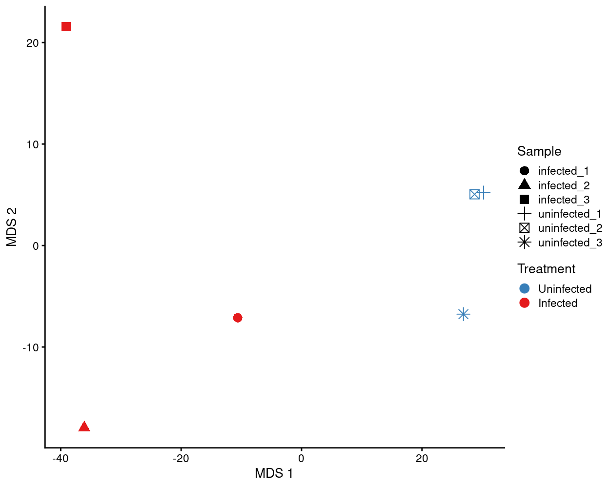
The results of this analysis are as if we had done a bulk RNA-seq experiment rather than scRNA-seq. It ignores the within-sample heterogeneity and consequently we recommend the results from the other differential analyses.

There is no DA analysis when ignoring cycling_subset.

DE

We require that a gene has an absolute fold change (\(FC\)) \(>1.5\) (i.e. \(|log_2(FC)| > log_2(1.5) \approx 0.58\)) and an \(FDR < 0.05\) to be called as differentially expressed. This is achieved by using the glmTreat() method in edgeR, which is a statistically rigorous method for thresholded differential expression testing.

Please see output/DEGs/cycling_subset/ for heatmaps and spreadsheets of these DEG lists, including results of GO and KEGG analyses using the goana() and kegga() functions from the limma package. The heatmaps show up to the top-50 DEGs (ordered by \(FDR\)).

This directory also contains interactive Glimma plots of the differential expression results. The Glimma plots show the pseudobulk data for that label.

Note that the DEG list spreadsheets contain all labels and genes whereas the Glimma plots only contain labels and genes actually tested for DE. The column names in the Glimma tables may be abbreviated. There are two types of heatmaps: (1) showing the ‘pseudobulk’ expression and (2) showing the average single-cell expression.

Show code

# NOTE: Have to drop the complicated TRA and TRB DFrameList objects.
x <- sce
x$TRA <- NULL
x$TRB <- NULL
sce.ignoring_cycling_subset <- aggregateAcrossCells(
  x,
  id = colData(x)[, c("Sample", "Treatment")],
  coldata.merge = FALSE,
  use.dimred = FALSE,
  use.altexps = FALSE)
sizeFactors(sce.ignoring_cycling_subset) <- NULL
sce.ignoring_cycling_subset <- logNormCounts(sce.ignoring_cycling_subset)
colLabels(sce.ignoring_cycling_subset) <- "ignoring_cycling_subset"
colnames(sce.ignoring_cycling_subset) <-
  paste0(colLabels(sce.ignoring_cycling_subset),
         ".",
         sce.ignoring_cycling_subset$Sample)

Show code

sce.ignoring_cycling_subset <- runMDS(sce.ignoring_cycling_subset)
plotMDS(
  sce.ignoring_cycling_subset,
  colour_by = "Treatment",
  shape_by = "Sample",
  point_size = 3,
  point_alpha = 2) +
  scale_colour_manual(values = treatment_colours, name = "Treatment")

Show code

sce.ignoring_cycling_subset_filt <-
  sce.ignoring_cycling_subset[, sce.ignoring_cycling_subset$ncells >= 10]

de_results <- pseudoBulkDGE(
  sce.ignoring_cycling_subset_filt,
  label = sce.ignoring_cycling_subset_filt$label,
  design = ~Treatment,
  coef = "TreatmentInfected",
  condition = sce.ignoring_cycling_subset_filt$Treatment,
  include.intermediates = TRUE,
  lfc = log2(1.5))

• Labels for which we couldn’t run DE (character(0) means none)

Show code

metadata(de_results)$failed

character(0)

• Number of DEGs per label (-1 means downregulated in Infected vs. Uninfected, 0 means not DE, 1 means upregulated in Infected vs. Uninfected)

Show code

is.de <- decideTestsPerLabel(de_results, threshold = 0.05)
summarizeTestsPerLabel(is.de)

                        -1     0  1   NA
ignoring_cycling_subset 74 11562 92 8874

Show code

outdir <- here("output", "DEGs", "ignoring_cycling_subset")
dir.create(outdir, recursive = TRUE)
createDEGOutputs(
  outdir = outdir,
  de_results = de_results,
  summed_filt = sce.ignoring_cycling_subset_filt,
  sce = sce,
  fdr = 0.05)

Show code

lapply(names(de_results), function(n) {
  se <- sce.ignoring_cycling_subset_filt[
    , sce.ignoring_cycling_subset_filt$label == n]
  x <- de_results[[n]]
  x <- x[order(x$FDR), ]
  features <- rownames(x[which(x$FDR < 0.05), ])
  if (length(features) > 2) {
    plotHeatmap(
      se,
      features = head(features, 50),
      center = TRUE,
      zlim = c(-3, 3),
      symmetric = TRUE,
      color = hcl.colors(101, "Blue-Red 3"),
      order_columns_by = c("Treatment", "Sample"),
      column_annotation_colors = list(
        Treatment = treatment_colours,
        Sample = sample_colours),
      cluster_rows = TRUE,
      fontsize = 8,
      main = n,
      filename = file.path(outdir, paste0(n, ".pseudobulk_heatmap.pdf")))

    plotGroupedHeatmap(
      sce,
      features = head(features, 50),
      group = "Sample",
      center = TRUE,
      symmetric = TRUE,
      color = hcl.colors(101, "Blue-Red 3"),
      cluster_rows = TRUE,
      fontsize = 8,
      main = n,
      cluster_cols = FALSE,
      filename = file.path(
        outdir,
        paste0(n, ".average_expression_heatmap.pdf")))
  }
})

Gene set testing

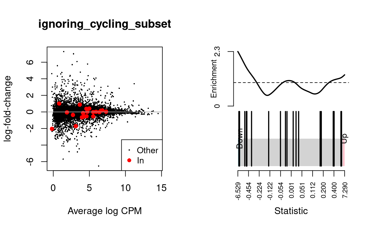
We use the fry() function from the edgeR R/Bioconductor package to perform a self-contained gene set test against the null hypothesis that none of the genes in the BCL-family gene set (supplied by James) are differentially expressed. We can visualise the expression of the genes in any given set and in any given comparison by highlighting those genes on the MD plot and/or using a ‘barcode plot.’ Such figures are often included in publications.

Show code

# NOTE: The following is a workaround to the lack of support for tabsets in 
#       distill (see https://github.com/rstudio/distill/issues/11 and 
#       https://github.com/rstudio/distill/issues/11#issuecomment-692142414 in 
#       particular).
xaringanExtra::use_panelset()

ignoring_cycling_subset

Show code

n <- "ignoring_cycling_subset"
md <- metadata(de_results[[n]])
y <- md$y
y_design <- md$design
y_index <- ids2indices(
  list(`BCL2-family` = bcl2_df$Approved.symbol),
  rownames(y))
fry(
  y,
  index = y_index,
  design = y_design,
  coef = "TreatmentInfected") %>%
  knitr::kable(
    caption = "Results of applying `fry()` to the RNA-seq differential expression results using the supplied gene sets. A significant 'Up' P-value means that the differential expression results found in the RNA-seq data are positively correlated with the expression signature from the corresponding gene set. Conversely, a significant 'Down' P-value means that the differential expression log-fold-changes are negatively correlated with the expression signature from the corresponding gene set. A significant 'Mixed' P-value means that the genes in the set tend to be differentially expressed without regard for direction.")

Table 1: Results of applying fry() to the RNA-seq differential expression results using the supplied gene sets. A significant ‘Up’ P-value means that the differential expression results found in the RNA-seq data are positively correlated with the expression signature from the corresponding gene set. Conversely, a significant ‘Down’ P-value means that the differential expression log-fold-changes are negatively correlated with the expression signature from the corresponding gene set. A significant ‘Mixed’ P-value means that the genes in the set tend to be differentially expressed without regard for direction.

	NGenes	Direction	PValue	PValue.Mixed
BCL2-family	20	Down	0.0624809	0.000225

Show code

dgelrt <- glmTreat(md$fit, coef = "TreatmentInfected", lfc = log2(1.5))
par(mfrow = c(1, 2))
y_status <- rep("Other", nrow(dgelrt))
y_status[rownames(dgelrt) %in% bcl2_df$Approved.symbol] <- "In"
plotMD(
  dgelrt,
  status = y_status,
  values = "In",
  hl.col = "red",
  legend = "bottomright",
  main = n)
abline(h = 0, col = "darkgrey")
barcodeplot(
  statistics = dgelrt$table$logFC,
  index = rownames(dgelrt) %in% bcl2_df$Approved.symbol)

Analysis based on cycling_subset

DE

We require that a gene has an absolute fold change (\(FC\)) \(>1.5\) (i.e. \(|log_2(FC)| > log_2(1.5) \approx 0.58\)) and an \(FDR < 0.05\) to be called as differentially expressed. This is achieved by using the glmTreat() method in edgeR, which is a statistically rigorous method for thresholded differential expression testing.

Please see output/DEGs/cycling_subset/ for heatmaps and spreadsheets of these DEG lists, including results of GO and KEGG analyses using the goana() and kegga() functions from the limma package. The heatmaps show up to the top-50 DEGs (ordered by \(FDR\)).

This directory also contains interactive Glimma plots of the differential expression results. The Glimma plots show the pseudobulk data for that label.

Note that the DEG list spreadsheets contain all labels and genes whereas the Glimma plots only contain labels and genes actually tested for DE. The column names in the Glimma tables may be abbreviated. There are two types of heatmaps: (1) showing the ‘pseudobulk’ expression and (2) showing the average single-cell expression.

Show code

# NOTE: Have to drop the complicated TRA and TRB DFrameList objects.
x <- sce
x$TRA <- NULL
x$TRB <- NULL
sce.cycling_subset_Sample <- aggregateAcrossCells(
  x,
  id = colData(x)[, c("cycling_subset", "Sample", "Treatment")],
  coldata.merge = FALSE,
  use.dimred = FALSE,
  use.altexps = FALSE)
sizeFactors(sce.cycling_subset_Sample) <- NULL
sce.cycling_subset_Sample <- logNormCounts(sce.cycling_subset_Sample)
colLabels(sce.cycling_subset_Sample) <- sce.cycling_subset_Sample$cycling_subset
colnames(sce.cycling_subset_Sample) <-
  paste0(sce.cycling_subset_Sample$cycling_subset,
         ".",
         sce.cycling_subset_Sample$Sample)

Show code

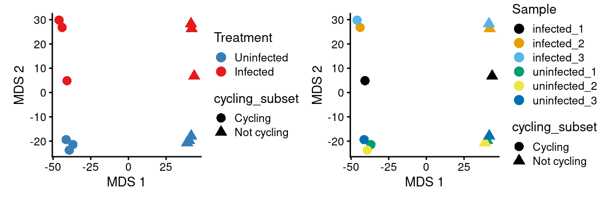
sce.cycling_subset_Sample <- runMDS(sce.cycling_subset_Sample)
p1 <- plotMDS(
  sce.cycling_subset_Sample,
  colour_by = "Treatment",
  shape_by = "cycling_subset",
  point_size = 3,
  point_alpha = 2) +
  scale_colour_manual(values = treatment_colours, name = "Treatment")
p2 <- plotMDS(
  sce.cycling_subset_Sample,
  colour_by = "Sample",
  shape_by = "cycling_subset",
  point_size = 3,
  point_alpha = 2) +
  scale_colour_manual(values = sample_colours, name = "Sample")
p1 + p2

Show code

sce.cycling_subset_Sample_filt <-
  sce.cycling_subset_Sample[, sce.cycling_subset_Sample$ncells >= 10]

de_results <- pseudoBulkDGE(
  sce.cycling_subset_Sample_filt,
  label = sce.cycling_subset_Sample_filt$cycling_subset,
  design = ~Treatment,
  coef = "TreatmentInfected",
  condition = sce.cycling_subset_Sample_filt$Treatment,
  include.intermediates = TRUE,
  lfc = log2(1.5))

• Labels for which we couldn’t run DE (character(0) means none)

Show code

metadata(de_results)$failed

character(0)

• Number of DEGs per label (-1 means downregulated in Infected vs. Uninfected, 0 means not DE, 1 means upregulated in Infected vs. Uninfected)

Show code

is.de <- decideTestsPerLabel(de_results, threshold = 0.05)
summarizeTestsPerLabel(is.de)

            -1     0  1    NA
Cycling     38  9799 53 10712
Not cycling 82 11016 97  9407

Show code

outdir <- here("output", "DEGs", "cycling_subset")
dir.create(outdir, recursive = TRUE)
createDEGOutputs(
  outdir = outdir,
  de_results = de_results,
  summed_filt = sce.cycling_subset_Sample_filt,
  sce = sce,
  fdr = 0.05)

Show code

lapply(names(de_results), function(n) {
  se <- sce.cycling_subset_Sample_filt[, sce.cycling_subset_Sample_filt$label == n]
  x <- de_results[[n]]
  x <- x[order(x$FDR), ]
  features <- rownames(x[which(x$FDR < 0.05), ])
  if (length(features) > 2) {
    plotHeatmap(
      se,
      features = head(features, 50),
      center = TRUE,
      zlim = c(-3, 3),
      symmetric = TRUE,
      color = hcl.colors(101, "Blue-Red 3"),
      order_columns_by = c("Treatment", "Sample"),
      column_annotation_colors = list(
        Treatment = treatment_colours,
        Sample = sample_colours),
      cluster_rows = TRUE,
      fontsize = 8,
      main = n,
      filename = file.path(outdir, paste0(n, ".pseudobulk_heatmap.pdf")))

    plotGroupedHeatmap(
      sce,
      features = head(features, 50),
      group = "Sample",
      columns = sce$cycling_subset == n,
      center = TRUE,
      symmetric = TRUE,
      color = hcl.colors(101, "Blue-Red 3"),
      cluster_rows = TRUE,
      fontsize = 8,
      main = n,
      cluster_cols = FALSE,
      filename = file.path(
        outdir,
        paste0(n, ".average_expression_heatmap.pdf")))
  }
})

Gene set testing

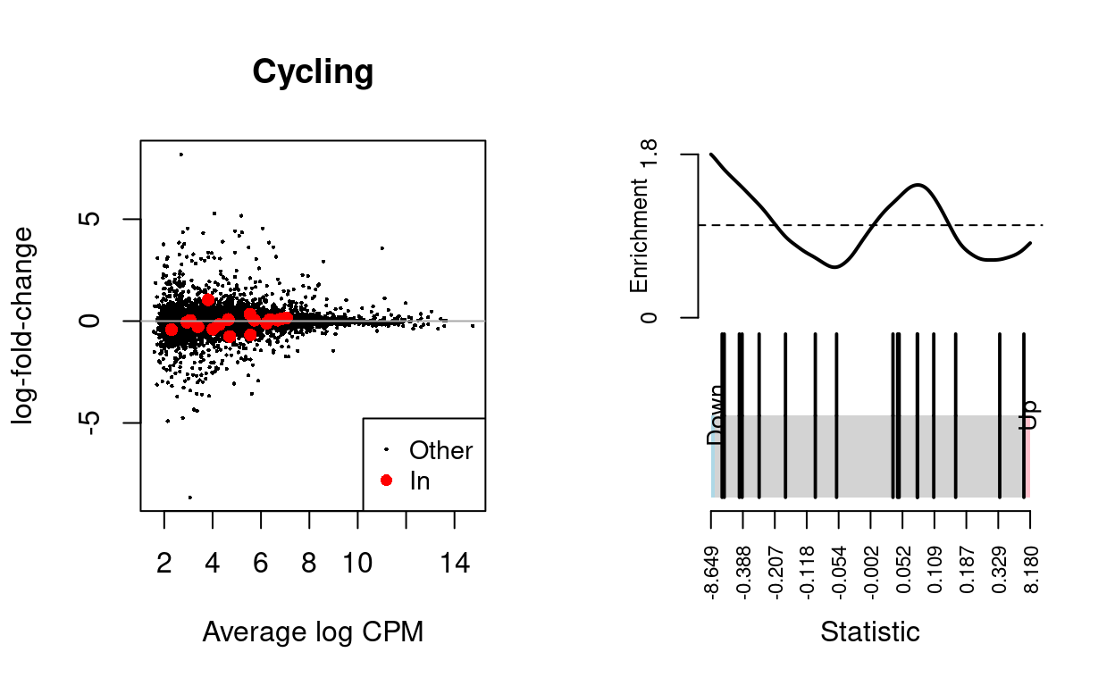
We use the fry() function from the edgeR R/Bioconductor package to perform a self-contained gene set test against the null hypothesis that none of the genes in the BCL-family gene set (supplied by James) are differentially expressed. We can visualise the expression of the genes in any given set and in any given comparison by highlighting those genes on the MD plot and/or using a ‘barcode plot.’ Such figures are often included in publications.

Cycling

Show code

n <- "Cycling"
md <- metadata(de_results[[n]])
y <- md$y
y_design <- md$design
y_index <- ids2indices(
  list(`BCL2-family` = bcl2_df$Approved.symbol),
  rownames(y))
fry(
  y,
  index = y_index,
  design = y_design,
  coef = "TreatmentInfected") %>%
  knitr::kable(
    caption = "Results of applying `fry()` to the RNA-seq differential expression results using the supplied gene sets. A significant 'Up' P-value means that the differential expression results found in the RNA-seq data are positively correlated with the expression signature from the corresponding gene set. Conversely, a significant 'Down' P-value means that the differential expression log-fold-changes are negatively correlated with the expression signature from the corresponding gene set. A significant 'Mixed' P-value means that the genes in the set tend to be differentially expressed without regard for direction.")

Table 2: Results of applying fry() to the RNA-seq differential expression results using the supplied gene sets. A significant ‘Up’ P-value means that the differential expression results found in the RNA-seq data are positively correlated with the expression signature from the corresponding gene set. Conversely, a significant ‘Down’ P-value means that the differential expression log-fold-changes are negatively correlated with the expression signature from the corresponding gene set. A significant ‘Mixed’ P-value means that the genes in the set tend to be differentially expressed without regard for direction.

	NGenes	Direction	PValue	PValue.Mixed
BCL2-family	17	Down	0.5963644	0.0048845

Show code

dgelrt <- glmTreat(md$fit, coef = "TreatmentInfected", lfc = log2(1.5))
par(mfrow = c(1, 2))
y_status <- rep("Other", nrow(dgelrt))
y_status[rownames(dgelrt) %in% bcl2_df$Approved.symbol] <- "In"
plotMD(
  dgelrt,
  status = y_status,
  values = "In",
  hl.col = "red",
  legend = "bottomright",
  main = n)
abline(h = 0, col = "darkgrey")
barcodeplot(
  statistics = dgelrt$table$logFC,
  index = rownames(dgelrt) %in% bcl2_df$Approved.symbol)

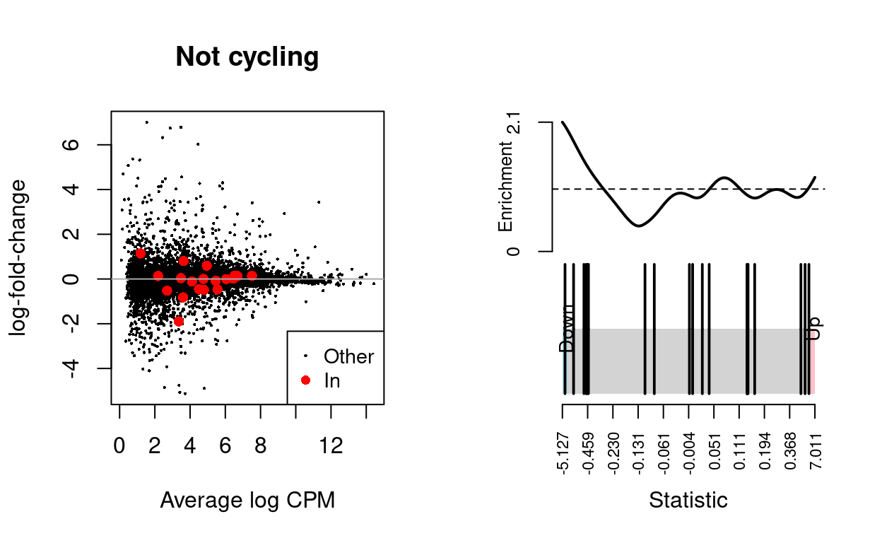
Not cycling

Show code

n <- "Not cycling"
md <- metadata(de_results[[n]])
y <- md$y
y_design <- md$design
y_index <- ids2indices(
  list(`BCL2-family` = bcl2_df$Approved.symbol),
  rownames(y))
fry(
  y,
  index = y_index,
  design = y_design,
  coef = "TreatmentInfected") %>%
  knitr::kable(
    caption = "Results of applying `fry()` to the RNA-seq differential expression results using the supplied gene sets. A significant 'Up' P-value means that the differential expression results found in the RNA-seq data are positively correlated with the expression signature from the corresponding gene set. Conversely, a significant 'Down' P-value means that the differential expression log-fold-changes are negatively correlated with the expression signature from the corresponding gene set. A significant 'Mixed' P-value means that the genes in the set tend to be differentially expressed without regard for direction.")

Table 3: Results of applying fry() to the RNA-seq differential expression results using the supplied gene sets. A significant ‘Up’ P-value means that the differential expression results found in the RNA-seq data are positively correlated with the expression signature from the corresponding gene set. Conversely, a significant ‘Down’ P-value means that the differential expression log-fold-changes are negatively correlated with the expression signature from the corresponding gene set. A significant ‘Mixed’ P-value means that the genes in the set tend to be differentially expressed without regard for direction.

	NGenes	Direction	PValue	PValue.Mixed
BCL2-family	19	Down	0.1278257	0.0002985

Show code

dgelrt <- glmTreat(md$fit, coef = "TreatmentInfected", lfc = log2(1.5))
par(mfrow = c(1, 2))
y_status <- rep("Other", nrow(dgelrt))
y_status[rownames(dgelrt) %in% bcl2_df$Approved.symbol] <- "In"
plotMD(
  dgelrt,
  status = y_status,
  values = "In",
  hl.col = "red",
  legend = "bottomright",
  main = n)
abline(h = 0, col = "darkgrey")
barcodeplot(
  statistics = dgelrt$table$logFC,
  index = rownames(dgelrt) %in% bcl2_df$Approved.symbol)

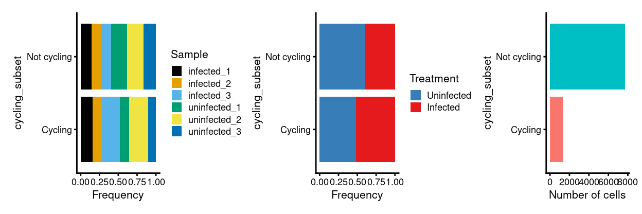
DA

• Number of cells/label/sample

Show code

abundances <- table(sce$cycling_subset, sce$Sample)
abundances <- unclass(abundances)
abundances

              infected_1 infected_2 infected_3 uninfected_1
  Cycling            226        171        327          171
  Not cycling       1121       1004       1007         1618

              uninfected_2 uninfected_3
  Cycling              358          142
  Not cycling         1694         1292

Show code

p1 <- plotUMAP(
  sce,
  colour_by = "cycling_subset",
  text_by = "cycling_subset",
  point_size = 0.5,
  point_alpha = 1,
  text_size = 4)
p2 <- plotUMAP(
  sce,
  colour_by = "Treatment",
  point_size = 0.5,
  point_alpha = 1) +
  scale_colour_manual(values = treatment_colours, name = "Treatment")
p1 + p2

Show code

p3 <- ggplot(as.data.frame(colData(sce)[, c("cycling_subset", "Sample")])) +
    geom_bar(
      aes(x = cycling_subset, fill = Sample),
      position = position_fill(reverse = TRUE)) +
    coord_flip() +
    ylab("Frequency") +
    scale_fill_manual(values = sample_colours) +
    theme_cowplot(font_size = 8)
p4 <- ggplot(as.data.frame(colData(sce)[, c("cycling_subset", "Treatment")])) +
    geom_bar(
      aes(x = cycling_subset, fill = Treatment),
      position = position_fill(reverse = TRUE)) +
    coord_flip() +
    ylab("Frequency") +
    scale_fill_manual(values = treatment_colours) +
    theme_cowplot(font_size = 8)
p5 <- ggplot(as.data.frame(colData(sce)[, "cycling_subset", drop = FALSE])) +
    geom_bar(aes(x = cycling_subset, fill = cycling_subset)) +
    coord_flip() +
    ylab("Number of cells") +
    theme_cowplot(font_size = 8) +
    guides(fill = FALSE)
p3 + p4 + p5 + plot_layout(ncol = 3)

• TRUE/FALSE if label can be tested for DA

Show code

# NOTE: Can't use quasi-likelihood framework with only two labels.

extra.info <- colData(sce)[match(colnames(abundances), sce$Sample), ]
y.ab <- DGEList(abundances, samples = extra.info)

keep <- filterByExpr(y.ab, group = y.ab$samples$Treatment)
keep

    Cycling Not cycling
       TRUE        TRUE 

• Number of labels that are DA (-1 means less abundant in Infected vs. Uninfected, 0 means not DE, 1 means more abundant in Infected vs. Uninfected)

Show code

y.ab <- y.ab[keep,]

design <- model.matrix(~Treatment, y.ab$samples)

y.ab <- estimateDisp(y.ab, design, trend = "none")
fit.ab <- glmFit(y.ab)
res <- glmLRT(fit.ab, coef = "TreatmentInfected")
summary(decideTests(res))

       TreatmentInfected
Down                   0
NotSig                 2
Up                     0

• Full results (negative logFC means less abundant in Infected vs. Uninfected, positive logFC means more abundant in Infected vs. Uninfected)

Show code

topTags(res, n = Inf)

Coefficient:  TreatmentInfected
                 logFC   logCPM       LR     PValue       FDR
Cycling      0.5952481 17.24486 2.947518 0.08600953 0.1720191
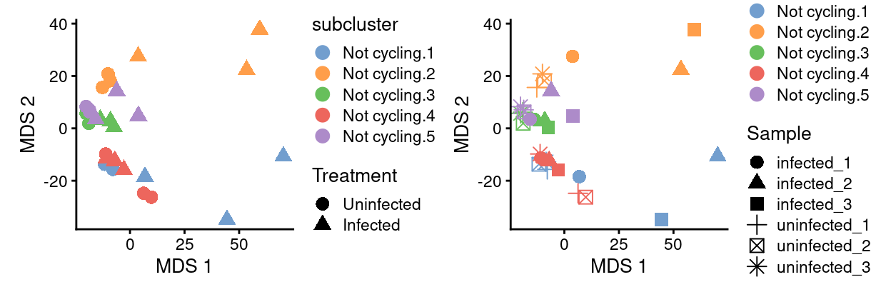
Not cycling -0.1075603 19.68781 1.001231 0.31701277 0.3170128

Analysis based on subcluster labels in Not cycling subset

DE

We require that a gene has an absolute fold change (\(FC\)) \(>1.5\) (i.e. \(|log_2(FC)| > log_2(1.5) \approx 0.58\)) and an \(FDR < 0.05\) to be called as differentially expressed. This is achieved by using the glmTreat() method in edgeR, which is a statistically rigorous method for thresholded differential expression testing.

Please see output/DEGs/not_cycling_subset_subclusters/ for heatmaps and spreadsheets of these DEG lists, including results of GO and KEGG analyses using the goana() and kegga() functions from the limma package. The heatmaps show up to the top-50 DEGs (ordered by \(FDR\)).

This directory also contains interactive Glimma plots of the differential expression results. The Glimma plots show the pseudobulk data for that label.

Note that the DEG list spreadsheets contain all labels and genes whereas the Glimma plots only contain labels and genes actually tested for DE. The column names in the Glimma tables may be abbreviated. There are two types of heatmaps: (1) showing the ‘pseudobulk’ expression and (2) showing the average single-cell expression.

Show code

# NOTE: Have to drop the complicated TRA and TRB DFrameList objects.
x <- not_cycling_sce
x$TRA <- NULL
x$TRB <- NULL
not_cycling_sce.subcluster_Sample <- aggregateAcrossCells(
  x,
  id = colData(x)[, c("subcluster", "Sample", "Treatment")],
  coldata.merge = FALSE,
  use.dimred = FALSE,
  use.altexps = FALSE)
sizeFactors(not_cycling_sce.subcluster_Sample) <- NULL
not_cycling_sce.subcluster_Sample <-
  logNormCounts(not_cycling_sce.subcluster_Sample)
colLabels(not_cycling_sce.subcluster_Sample) <-
  not_cycling_sce.subcluster_Sample$subcluster
colnames(not_cycling_sce.subcluster_Sample) <- paste0(
  not_cycling_sce.subcluster_Sample$subcluster,
  ".",
  not_cycling_sce.subcluster_Sample$Sample)

Show code

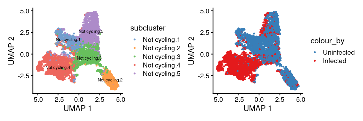
not_cycling_sce.subcluster_Sample <- runMDS(not_cycling_sce.subcluster_Sample)
p1 <- plotMDS(
  not_cycling_sce.subcluster_Sample,
  colour_by = "subcluster",
  shape_by = "Treatment",
  point_size = 3,
  point_alpha = 2)
p2 <- plotMDS(
  not_cycling_sce.subcluster_Sample,
  colour_by = "subcluster",
  shape_by = "Sample",
  point_size = 3,
  point_alpha = 2)
p1 + p2

Show code

not_cycling_sce.subcluster_Sample_filt <-
  not_cycling_sce.subcluster_Sample[, not_cycling_sce.subcluster_Sample$ncells >= 10]

de_results <- pseudoBulkDGE(
  not_cycling_sce.subcluster_Sample_filt,
  label = not_cycling_sce.subcluster_Sample_filt$subcluster,
  design = ~Treatment,
  coef = "TreatmentInfected",
  condition = not_cycling_sce.subcluster_Sample_filt$Treatment,
  include.intermediates = TRUE,
  lfc = log2(1.5))

• Labels for which we couldn’t run DE (character(0) means none)

Show code

metadata(de_results)$failed

character(0)

• Number of DEGs per label (-1 means downregulated in Infected vs. Uninfected, 0 means not DE, 1 means upregulated in Infected vs. Uninfected)

Show code

is.de <- decideTestsPerLabel(de_results, threshold = 0.05)
summarizeTestsPerLabel(is.de)

              -1    0  1    NA
Not cycling.1  1 6120  0 14481
Not cycling.2  2 8254  5 12341
Not cycling.3 10 8829 25 11738
Not cycling.4  3 9086  0 11513
Not cycling.5  3 9465 27 11107

Show code

outdir <- here("output", "DEGs", "not_cycling_subset_subcluster")
dir.create(outdir, recursive = TRUE)
createDEGOutputs(
  outdir = outdir,
  de_results = de_results,
  summed_filt = not_cycling_sce.subcluster_Sample_filt,
  sce = x,
  fdr = 0.05)

Show code

lapply(names(de_results), function(n) {
  se <- not_cycling_sce.subcluster_Sample_filt[, not_cycling_sce.subcluster_Sample_filt$label == n]
  x <- de_results[[n]]
  x <- x[order(x$FDR), ]
  features <- rownames(x[which(x$FDR < 0.05), ])
  if (length(features) > 2) {
    plotHeatmap(
      se,
      features = head(features, 50),
      center = TRUE,
      zlim = c(-3, 3),
      symmetric = TRUE,
      color = hcl.colors(101, "Blue-Red 3"),
      order_columns_by = c("Treatment", "Sample"),
      column_annotation_colors = list(
        Treatment = treatment_colours,
        Sample = sample_colours),
      cluster_rows = TRUE,
      fontsize = 8,
      main = n,
      filename = file.path(outdir, paste0(n, ".pseudobulk_heatmap.pdf")))

    plotGroupedHeatmap(
      not_cycling_sce,
      features = head(features, 50),
      group = "Sample",
      columns = not_cycling_sce$subcluster == n,
      center = TRUE,
      symmetric = TRUE,
      color = hcl.colors(101, "Blue-Red 3"),
      cluster_rows = TRUE,
      fontsize = 8,
      main = n,
      cluster_cols = FALSE,
      filename = file.path(
        outdir,
        paste0(n, ".average_expression_heatmap.pdf")))
  }
})

Gene set testing

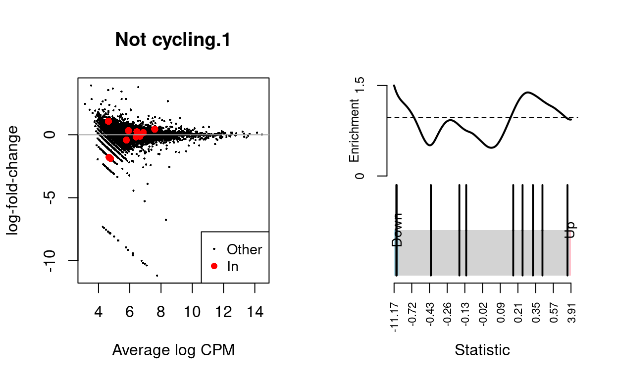
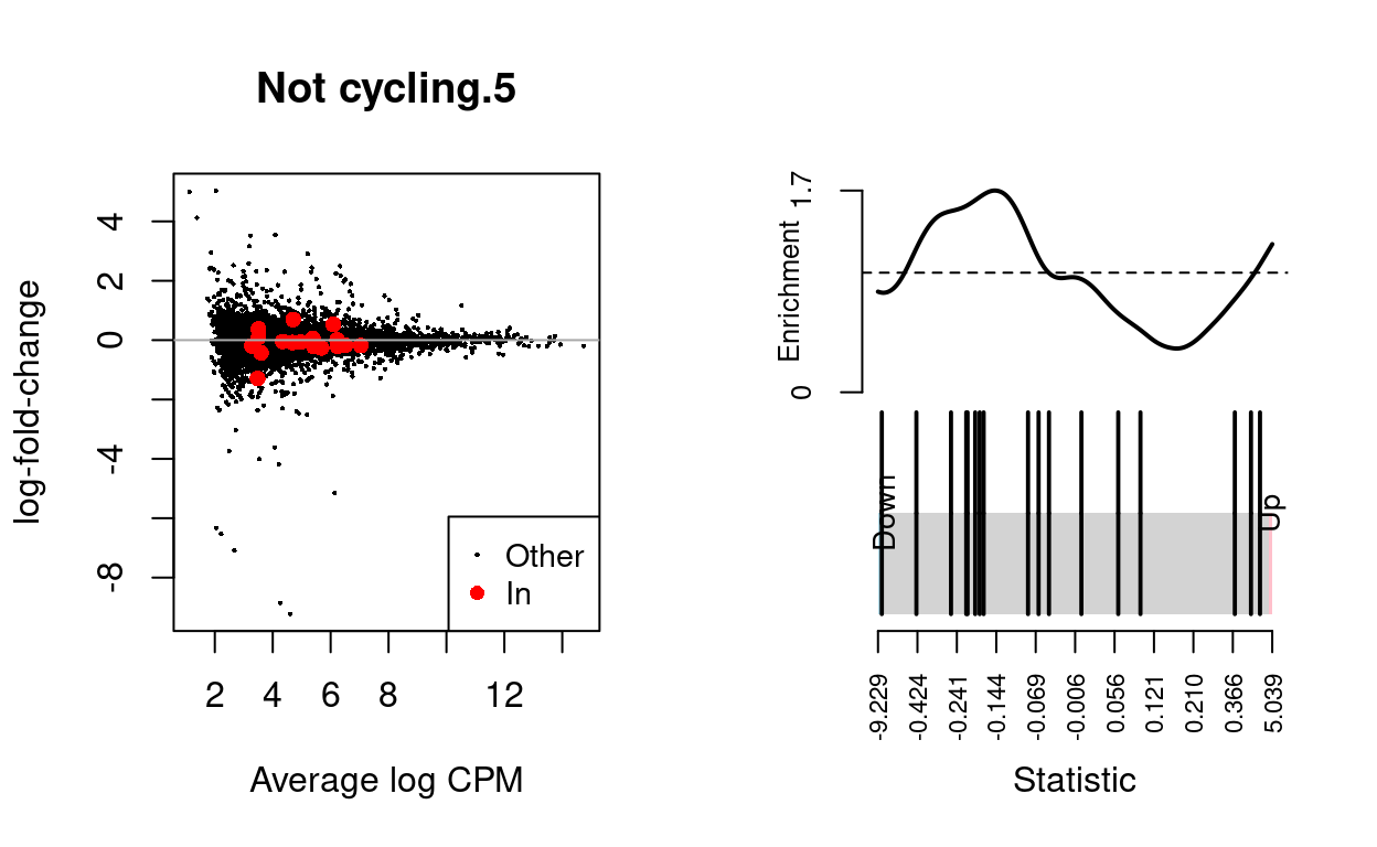
We use the fry() function from the edgeR R/Bioconductor package to perform a self-contained gene set test against the null hypothesis that none of the genes in the BCL-family gene set (supplied by James) are differentially expressed. We can visualise the expression of the genes in any given set and in any given comparison by highlighting those genes on the MD plot and/or using a ‘barcode plot.’ Such figures are often included in publications.

Not cycling.1

Show code

n <- "Not cycling.1"
md <- metadata(de_results[[n]])
y <- md$y
y_design <- md$design
y_index <- ids2indices(
  list(`BCL2-family` = bcl2_df$Approved.symbol),
  rownames(y))
fry(
  y,
  index = y_index,
  design = y_design,
  coef = "TreatmentInfected") %>%
  knitr::kable(
    caption = "Results of applying `fry()` to the RNA-seq differential expression results using the supplied gene sets. A significant 'Up' P-value means that the differential expression results found in the RNA-seq data are positively correlated with the expression signature from the corresponding gene set. Conversely, a significant 'Down' P-value means that the differential expression log-fold-changes are negatively correlated with the expression signature from the corresponding gene set. A significant 'Mixed' P-value means that the genes in the set tend to be differentially expressed without regard for direction.")

Table 4: Results of applying fry() to the RNA-seq differential expression results using the supplied gene sets. A significant ‘Up’ P-value means that the differential expression results found in the RNA-seq data are positively correlated with the expression signature from the corresponding gene set. Conversely, a significant ‘Down’ P-value means that the differential expression log-fold-changes are negatively correlated with the expression signature from the corresponding gene set. A significant ‘Mixed’ P-value means that the genes in the set tend to be differentially expressed without regard for direction.

	NGenes	Direction	PValue	PValue.Mixed
BCL2-family	10	Up	0.7725256	0.1818233

Show code

dgelrt <- glmTreat(md$fit, coef = "TreatmentInfected", lfc = log2(1.5))
par(mfrow = c(1, 2))
y_status <- rep("Other", nrow(dgelrt))
y_status[rownames(dgelrt) %in% bcl2_df$Approved.symbol] <- "In"
plotMD(
  dgelrt,
  status = y_status,
  values = "In",
  hl.col = "red",
  legend = "bottomright",
  main = n)
abline(h = 0, col = "darkgrey")
barcodeplot(
  statistics = dgelrt$table$logFC,
  index = rownames(dgelrt) %in% bcl2_df$Approved.symbol)

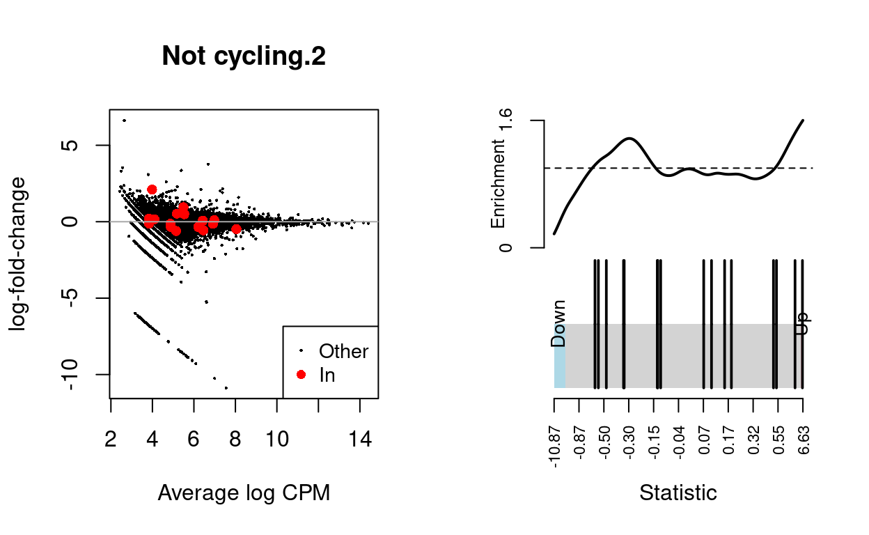
Not cycling.2

Show code

n <- "Not cycling.2"
md <- metadata(de_results[[n]])
y <- md$y
y_design <- md$design
y_index <- ids2indices(
  list(`BCL2-family` = bcl2_df$Approved.symbol),
  rownames(y))
fry(
  y,
  index = y_index,
  design = y_design,
  coef = "TreatmentInfected") %>%
  knitr::kable(
    caption = "Results of applying `fry()` to the RNA-seq differential expression results using the supplied gene sets. A significant 'Up' P-value means that the differential expression results found in the RNA-seq data are positively correlated with the expression signature from the corresponding gene set. Conversely, a significant 'Down' P-value means that the differential expression log-fold-changes are negatively correlated with the expression signature from the corresponding gene set. A significant 'Mixed' P-value means that the genes in the set tend to be differentially expressed without regard for direction.")

Table 5: Results of applying fry() to the RNA-seq differential expression results using the supplied gene sets. A significant ‘Up’ P-value means that the differential expression results found in the RNA-seq data are positively correlated with the expression signature from the corresponding gene set. Conversely, a significant ‘Down’ P-value means that the differential expression log-fold-changes are negatively correlated with the expression signature from the corresponding gene set. A significant ‘Mixed’ P-value means that the genes in the set tend to be differentially expressed without regard for direction.

	NGenes	Direction	PValue	PValue.Mixed
BCL2-family	16	Up	0.5962283	0.1791845

Show code

dgelrt <- glmTreat(md$fit, coef = "TreatmentInfected", lfc = log2(1.5))
par(mfrow = c(1, 2))
y_status <- rep("Other", nrow(dgelrt))
y_status[rownames(dgelrt) %in% bcl2_df$Approved.symbol] <- "In"
plotMD(
  dgelrt,
  status = y_status,
  values = "In",
  hl.col = "red",
  legend = "bottomright",
  main = n)
abline(h = 0, col = "darkgrey")
barcodeplot(
  statistics = dgelrt$table$logFC,
  index = rownames(dgelrt) %in% bcl2_df$Approved.symbol)

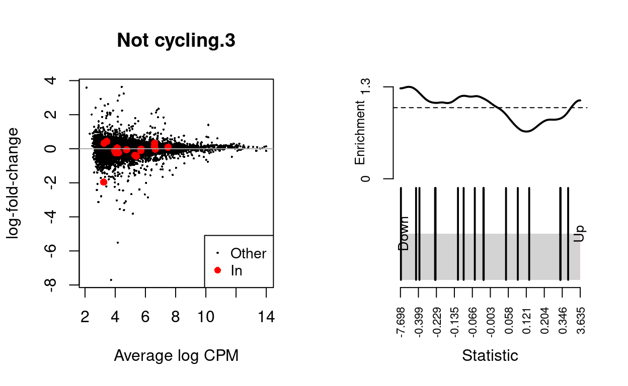
Not cycling.3

Show code

n <- "Not cycling.3"
md <- metadata(de_results[[n]])
y <- md$y
y_design <- md$design
y_index <- ids2indices(
  list(`BCL2-family` = bcl2_df$Approved.symbol),
  rownames(y))
fry(
  y,
  index = y_index,
  design = y_design,
  coef = "TreatmentInfected") %>%
  knitr::kable(
    caption = "Results of applying `fry()` to the RNA-seq differential expression results using the supplied gene sets. A significant 'Up' P-value means that the differential expression results found in the RNA-seq data are positively correlated with the expression signature from the corresponding gene set. Conversely, a significant 'Down' P-value means that the differential expression log-fold-changes are negatively correlated with the expression signature from the corresponding gene set. A significant 'Mixed' P-value means that the genes in the set tend to be differentially expressed without regard for direction.")

Table 6: Results of applying fry() to the RNA-seq differential expression results using the supplied gene sets. A significant ‘Up’ P-value means that the differential expression results found in the RNA-seq data are positively correlated with the expression signature from the corresponding gene set. Conversely, a significant ‘Down’ P-value means that the differential expression log-fold-changes are negatively correlated with the expression signature from the corresponding gene set. A significant ‘Mixed’ P-value means that the genes in the set tend to be differentially expressed without regard for direction.

	NGenes	Direction	PValue	PValue.Mixed
BCL2-family	16	Down	0.5429568	0.1337415

Show code

dgelrt <- glmTreat(md$fit, coef = "TreatmentInfected", lfc = log2(1.5))
par(mfrow = c(1, 2))
y_status <- rep("Other", nrow(dgelrt))
y_status[rownames(dgelrt) %in% bcl2_df$Approved.symbol] <- "In"
plotMD(
  dgelrt,
  status = y_status,
  values = "In",
  hl.col = "red",
  legend = "bottomright",
  main = n)
abline(h = 0, col = "darkgrey")
barcodeplot(
  statistics = dgelrt$table$logFC,
  index = rownames(dgelrt) %in% bcl2_df$Approved.symbol)

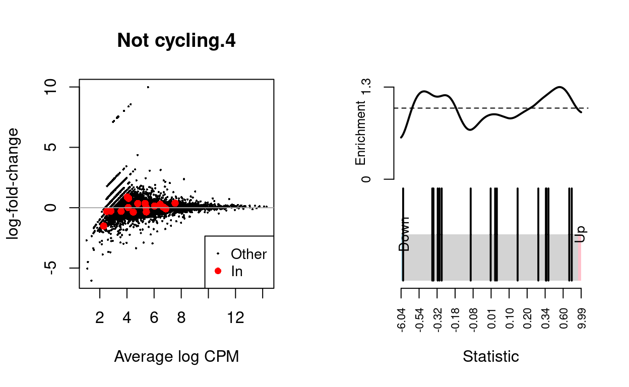
Not cycling.4

Show code

n <- "Not cycling.4"
md <- metadata(de_results[[n]])
y <- md$y
y_design <- md$design
y_index <- ids2indices(
  list(`BCL2-family` = bcl2_df$Approved.symbol),
  rownames(y))
fry(
  y,
  index = y_index,
  design = y_design,
  coef = "TreatmentInfected") %>%
  knitr::kable(
    caption = "Results of applying `fry()` to the RNA-seq differential expression results using the supplied gene sets. A significant 'Up' P-value means that the differential expression results found in the RNA-seq data are positively correlated with the expression signature from the corresponding gene set. Conversely, a significant 'Down' P-value means that the differential expression log-fold-changes are negatively correlated with the expression signature from the corresponding gene set. A significant 'Mixed' P-value means that the genes in the set tend to be differentially expressed without regard for direction.")

Table 7: Results of applying fry() to the RNA-seq differential expression results using the supplied gene sets. A significant ‘Up’ P-value means that the differential expression results found in the RNA-seq data are positively correlated with the expression signature from the corresponding gene set. Conversely, a significant ‘Down’ P-value means that the differential expression log-fold-changes are negatively correlated with the expression signature from the corresponding gene set. A significant ‘Mixed’ P-value means that the genes in the set tend to be differentially expressed without regard for direction.

	NGenes	Direction	PValue	PValue.Mixed
BCL2-family	17	Up	0.5591755	0.1480697

Show code

dgelrt <- glmTreat(md$fit, coef = "TreatmentInfected", lfc = log2(1.5))
par(mfrow = c(1, 2))
y_status <- rep("Other", nrow(dgelrt))
y_status[rownames(dgelrt) %in% bcl2_df$Approved.symbol] <- "In"
plotMD(
  dgelrt,
  status = y_status,
  values = "In",
  hl.col = "red",
  legend = "bottomright",
  main = n)
abline(h = 0, col = "darkgrey")
barcodeplot(
  statistics = dgelrt$table$logFC,
  index = rownames(dgelrt) %in% bcl2_df$Approved.symbol)

Not cycling.5

Show code

n <- "Not cycling.5"
md <- metadata(de_results[[n]])
y <- md$y
y_design <- md$design
y_index <- ids2indices(
  list(`BCL2-family` = bcl2_df$Approved.symbol),
  rownames(y))
fry(
  y,
  index = y_index,
  design = y_design,
  coef = "TreatmentInfected") %>%
  knitr::kable(
    caption = "Results of applying `fry()` to the RNA-seq differential expression results using the supplied gene sets. A significant 'Up' P-value means that the differential expression results found in the RNA-seq data are positively correlated with the expression signature from the corresponding gene set. Conversely, a significant 'Down' P-value means that the differential expression log-fold-changes are negatively correlated with the expression signature from the corresponding gene set. A significant 'Mixed' P-value means that the genes in the set tend to be differentially expressed without regard for direction.")

Table 8: Results of applying fry() to the RNA-seq differential expression results using the supplied gene sets. A significant ‘Up’ P-value means that the differential expression results found in the RNA-seq data are positively correlated with the expression signature from the corresponding gene set. Conversely, a significant ‘Down’ P-value means that the differential expression log-fold-changes are negatively correlated with the expression signature from the corresponding gene set. A significant ‘Mixed’ P-value means that the genes in the set tend to be differentially expressed without regard for direction.

	NGenes	Direction	PValue	PValue.Mixed
BCL2-family	17	Down	0.2202029	0.0323618

Show code

dgelrt <- glmTreat(md$fit, coef = "TreatmentInfected", lfc = log2(1.5))
par(mfrow = c(1, 2))
y_status <- rep("Other", nrow(dgelrt))
y_status[rownames(dgelrt) %in% bcl2_df$Approved.symbol] <- "In"
plotMD(
  dgelrt,
  status = y_status,
  values = "In",
  hl.col = "red",
  legend = "bottomright",
  main = n)
abline(h = 0, col = "darkgrey")
barcodeplot(
  statistics = dgelrt$table$logFC,
  index = rownames(dgelrt) %in% bcl2_df$Approved.symbol)

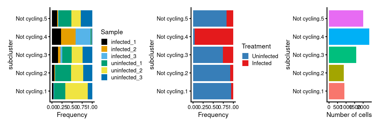
DA

• Number of cells/label/sample

Show code

abundances <- table(x$subcluster, x$Sample)
abundances <- unclass(abundances)
abundances

                infected_1 infected_2 infected_3 uninfected_1
  Not cycling.1         32          3         14          247
  Not cycling.2         53         11          7          342
  Not cycling.3        241        101         70          366
  Not cycling.4        532        848        881           29
  Not cycling.5        263         41         35          634

                uninfected_2 uninfected_3
  Not cycling.1          507           97
  Not cycling.2          258          197
  Not cycling.3          440          380
  Not cycling.4           30           41
  Not cycling.5          459          577

Show code

p1 <- plotUMAP(
  x,
  colour_by = "subcluster",
  text_by = "subcluster",
  point_size = 0.5,
  point_alpha = 1,
  text_size = 2)
p2 <- plotUMAP(
  x,
  colour_by = "Treatment",
  point_size = 0.5,
  point_alpha = 1) +
  scale_colour_manual(values = treatment_colours)
p1 + p2

Show code

p3 <- ggplot(as.data.frame(colData(x)[, c("subcluster", "Sample")])) +
  geom_bar(
    aes(x = subcluster, fill = Sample),
    position = position_fill(reverse = TRUE)) +
  coord_flip() +
  ylab("Frequency") +
  scale_fill_manual(values = sample_colours) +
  theme_cowplot(font_size = 8)
p4 <- ggplot(as.data.frame(colData(x)[, c("subcluster", "Treatment")])) +
  geom_bar(
    aes(x = subcluster, fill = Treatment),
    position = position_fill(reverse = TRUE)) +
  coord_flip() +
  ylab("Frequency") +
  scale_fill_manual(values = treatment_colours) +
  theme_cowplot(font_size = 8)
p5 <- ggplot(as.data.frame(colData(x)[, "subcluster", drop = FALSE])) +
  geom_bar(aes(x = subcluster, fill = subcluster)) +
  coord_flip() +
  ylab("Number of cells") +
  theme_cowplot(font_size = 8) +
  guides(fill = FALSE)
p3 + p4 + p5 + plot_layout(ncol = 3)

• TRUE/FALSE if label can be tested for DA

Show code

extra.info <- colData(sce)[match(colnames(abundances), sce$Sample), ]
y.ab <- DGEList(abundances, samples = extra.info)

keep <- filterByExpr(y.ab, group = y.ab$samples$Treatment)
keep

Not cycling.1 Not cycling.2 Not cycling.3 Not cycling.4 Not cycling.5
         TRUE          TRUE          TRUE          TRUE          TRUE 

• Number of labels that are DA (-1 means less abundant in Infected vs. Uninfected, 0 means not DE, 1 means more abundant in Infected vs. Uninfected)

Show code

y.ab <- y.ab[keep,]

design <- model.matrix(~Treatment, y.ab$samples)

y.ab <- estimateDisp(y.ab, design, trend = "none")
fit.ab <- glmFit(y.ab)
res <- glmLRT(fit.ab, coef = "TreatmentInfected")
summary(decideTests(res))

       TreatmentInfected
Down                   3
NotSig                 1
Up                     1

• Full results (negative logFC means less abundant in Infected vs. Uninfected, positive logFC means more abundant in Infected vs. Uninfected)

Show code

topTags(res, n = Inf)

Coefficient:  TreatmentInfected
                  logFC   logCPM        LR       PValue          FDR
Not cycling.4  5.023174 18.52370 35.433894 2.638552e-09 1.319276e-08
Not cycling.1 -3.521606 16.56704 19.295114 1.119926e-05 2.799814e-05
Not cycling.2 -2.973163 16.58736 14.604386 1.326055e-04 2.210092e-04
Not cycling.5 -1.835740 17.85842  6.212515 1.268503e-02 1.585629e-02
Not cycling.3 -1.017010 17.57522  2.006615 1.566145e-01 1.566145e-01

Analysis based on subcluster labels in Cycling subset

DE

We require that a gene has an absolute fold change (\(FC\)) \(>1.5\) (i.e. \(|log_2(FC)| > log_2(1.5) \approx 0.58\)) and an \(FDR < 0.05\) to be called as differentially expressed. This is achieved by using the glmTreat() method in edgeR, which is a statistically rigorous method for thresholded differential expression testing.

Please see output/DEGs/cycling_subset_subclusters/ for heatmaps and spreadsheets of these DEG lists, including results of GO and KEGG analyses using the goana() and kegga() functions from the limma package. The heatmaps show up to the top-50 DEGs (ordered by \(FDR\)).

This directory also contains interactive Glimma plots of the differential expression results. The Glimma plots show the pseudobulk data for that label.

Note that the DEG list spreadsheets contain all labels and genes whereas the Glimma plots only contain labels and genes actually tested for DE. The column names in the Glimma tables may be abbreviated. There are two types of heatmaps: (1) showing the ‘pseudobulk’ expression and (2) showing the average single-cell expression.

Show code

# NOTE: Have to drop the complicated TRA and TRB DFrameList objects.
x <- cycling_sce
x$TRA <- NULL
x$TRB <- NULL
cycling_sce.subcluster_Sample <- aggregateAcrossCells(
  x,
  id = colData(x)[, c("subcluster", "Sample", "Treatment")],
  coldata.merge = FALSE,
  use.dimred = FALSE,
  use.altexps = FALSE)
sizeFactors(cycling_sce.subcluster_Sample) <- NULL
cycling_sce.subcluster_Sample <- logNormCounts(cycling_sce.subcluster_Sample)
colLabels(cycling_sce.subcluster_Sample) <-
  cycling_sce.subcluster_Sample$subcluster
colnames(cycling_sce.subcluster_Sample) <- paste0(
  cycling_sce.subcluster_Sample$subcluster,
  ".",
  cycling_sce.subcluster_Sample$Sample)

Show code

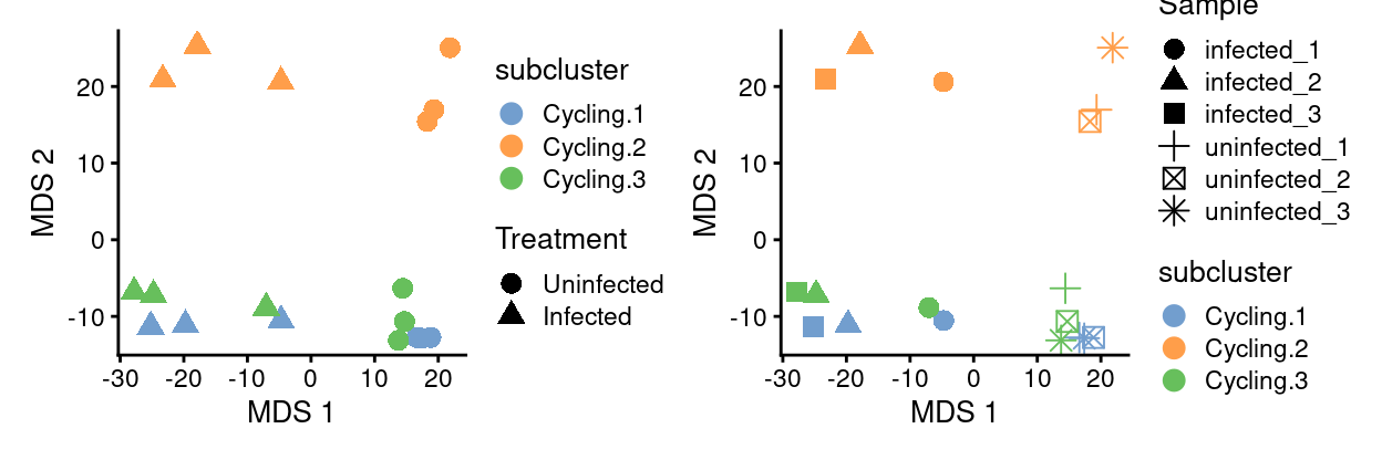
cycling_sce.subcluster_Sample <- runMDS(cycling_sce.subcluster_Sample)
p1 <- plotMDS(
  cycling_sce.subcluster_Sample,
  colour_by = "subcluster",
  shape_by = "Treatment",
  point_size = 3,
  point_alpha = 2)
p2 <- plotMDS(
  cycling_sce.subcluster_Sample,
  colour_by = "subcluster",
  shape_by = "Sample",
  point_size = 3,
  point_alpha = 2)
p1 + p2

Show code

cycling_sce.subcluster_Sample_filt <-
  cycling_sce.subcluster_Sample[, cycling_sce.subcluster_Sample$ncells >= 10]

de_results <- pseudoBulkDGE(
  cycling_sce.subcluster_Sample_filt,
  label = cycling_sce.subcluster_Sample_filt$subcluster,
  design = ~Treatment,
  coef = "TreatmentInfected",
  condition = cycling_sce.subcluster_Sample_filt$Treatment,
  include.intermediates = TRUE,
  lfc = log2(1.5))

• Labels for which we couldn’t run DE (character(0) means none)

Show code

metadata(de_results)$failed

character(0)

• Number of DEGs per label (-1 means downregulated in Infected vs. Uninfected, 0 means not DE, 1 means upregulated in Infected vs. Uninfected)

Show code

is.de <- decideTestsPerLabel(de_results, threshold = 0.05)
summarizeTestsPerLabel(is.de)

          -1    0  1    NA
Cycling.1 27 7659 29 12887
Cycling.2 11 6184 20 14387
Cycling.3 14 8500 29 12059

Show code

outdir <- here("output", "DEGs", "cycling_subset_subcluster")
dir.create(outdir, recursive = TRUE)
createDEGOutputs(
  outdir = outdir,
  de_results = de_results,
  summed_filt = cycling_sce.subcluster_Sample_filt,
  sce = x,
  fdr = 0.05)

Show code

lapply(names(de_results), function(n) {
  se <- cycling_sce.subcluster_Sample_filt[, cycling_sce.subcluster_Sample_filt$label == n]
  x <- de_results[[n]]
  x <- x[order(x$FDR), ]
  features <- rownames(x[which(x$FDR < 0.05), ])
  if (length(features) > 2) {
    plotHeatmap(
      se,
      features = head(features, 50),
      center = TRUE,
      zlim = c(-3, 3),
      symmetric = TRUE,
      color = hcl.colors(101, "Blue-Red 3"),
      order_columns_by = c("Treatment", "Sample"),
      column_annotation_colors = list(
        Treatment = treatment_colours,
        Sample = sample_colours),
      cluster_rows = TRUE,
      fontsize = 8,
      main = n,
      filename = file.path(outdir, paste0(n, ".pseudobulk_heatmap.pdf")))

    plotGroupedHeatmap(
      cycling_sce,
      features = head(features, 50),
      group = "Sample",
      columns = cycling_sce$subcluster == n,
      center = TRUE,
      symmetric = TRUE,
      color = hcl.colors(101, "Blue-Red 3"),
      cluster_rows = TRUE,
      fontsize = 8,
      main = n,
      cluster_cols = FALSE,
      filename = file.path(
        outdir,
        paste0(n, ".average_expression_heatmap.pdf")))
  }
})

Gene set testing

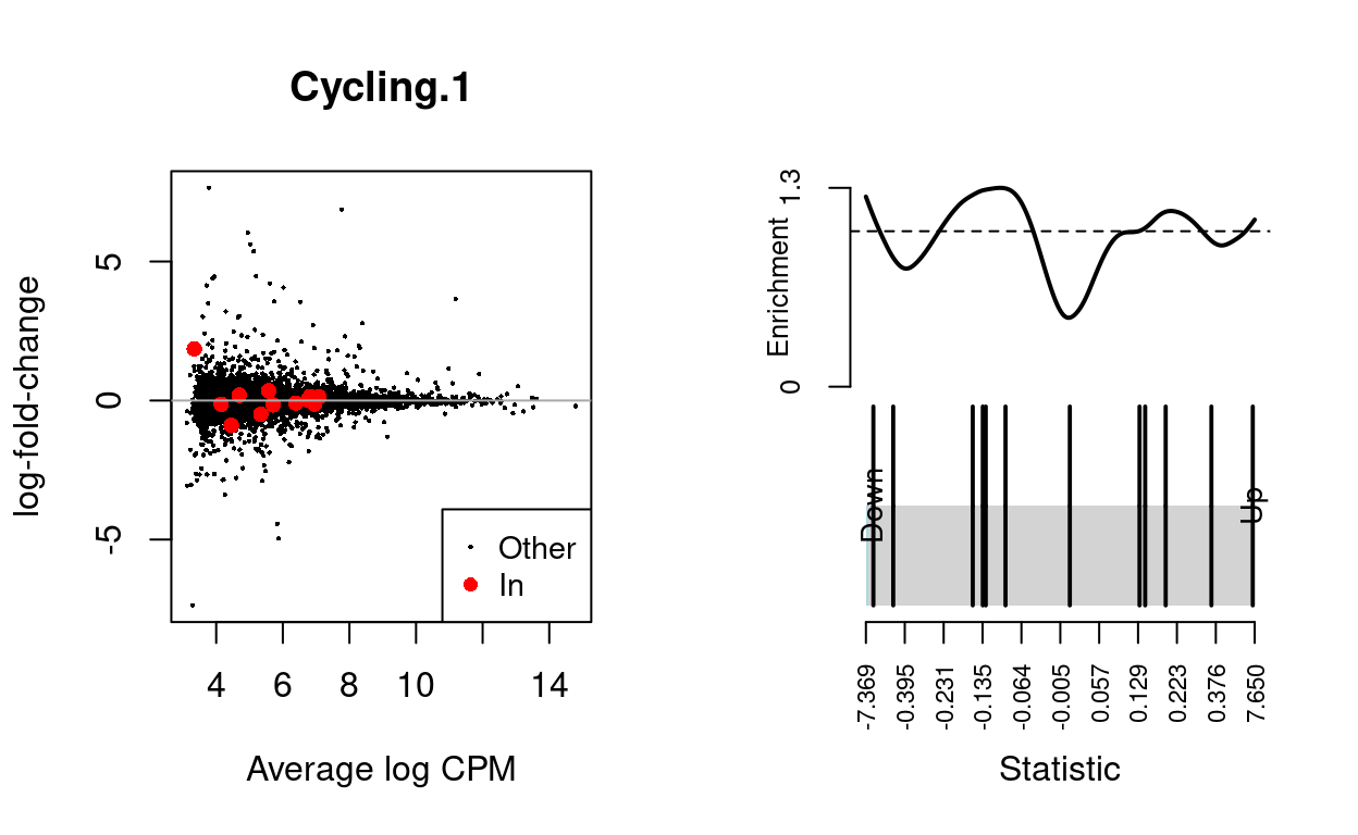
We use the fry() function from the edgeR R/Bioconductor package to perform a self-contained gene set test against the null hypothesis that none of the genes in the BCL-family gene set (supplied by James) are differentially expressed. We can visualise the expression of the genes in any given set and in any given comparison by highlighting those genes on the MD plot and/or using a ‘barcode plot.’ Such figures are often included in publications.

Cycling.1

Show code

n <- "Cycling.1"
md <- metadata(de_results[[n]])
y <- md$y
y_design <- md$design
y_index <- ids2indices(
  list(`BCL2-family` = bcl2_df$Approved.symbol),
  rownames(y))
fry(
  y,
  index = y_index,
  design = y_design,
  coef = "TreatmentInfected") %>%
  knitr::kable(
    caption = "Results of applying `fry()` to the RNA-seq differential expression results using the supplied gene sets. A significant 'Up' P-value means that the differential expression results found in the RNA-seq data are positively correlated with the expression signature from the corresponding gene set. Conversely, a significant 'Down' P-value means that the differential expression log-fold-changes are negatively correlated with the expression signature from the corresponding gene set. A significant 'Mixed' P-value means that the genes in the set tend to be differentially expressed without regard for direction.")

Table 9: Results of applying fry() to the RNA-seq differential expression results using the supplied gene sets. A significant ‘Up’ P-value means that the differential expression results found in the RNA-seq data are positively correlated with the expression signature from the corresponding gene set. Conversely, a significant ‘Down’ P-value means that the differential expression log-fold-changes are negatively correlated with the expression signature from the corresponding gene set. A significant ‘Mixed’ P-value means that the genes in the set tend to be differentially expressed without regard for direction.

	NGenes	Direction	PValue	PValue.Mixed
BCL2-family	12	Up	0.7233728	0.0026638

Show code

dgelrt <- glmTreat(md$fit, coef = "TreatmentInfected", lfc = log2(1.5))
par(mfrow = c(1, 2))
y_status <- rep("Other", nrow(dgelrt))
y_status[rownames(dgelrt) %in% bcl2_df$Approved.symbol] <- "In"
plotMD(
  dgelrt,
  status = y_status,
  values = "In",
  hl.col = "red",
  legend = "bottomright",
  main = n)
abline(h = 0, col = "darkgrey")
barcodeplot(
  statistics = dgelrt$table$logFC,
  index = rownames(dgelrt) %in% bcl2_df$Approved.symbol)

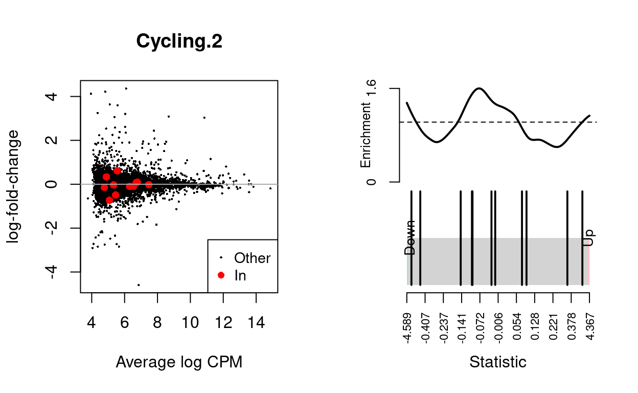
Cycling.2

Show code

n <- "Cycling.2"
md <- metadata(de_results[[n]])
y <- md$y
y_design <- md$design
y_index <- ids2indices(
  list(`BCL2-family` = bcl2_df$Approved.symbol),
  rownames(y))
fry(
  y,
  index = y_index,
  design = y_design,
  coef = "TreatmentInfected") %>%
  knitr::kable(
    caption = "Results of applying `fry()` to the RNA-seq differential expression results using the supplied gene sets. A significant 'Up' P-value means that the differential expression results found in the RNA-seq data are positively correlated with the expression signature from the corresponding gene set. Conversely, a significant 'Down' P-value means that the differential expression log-fold-changes are negatively correlated with the expression signature from the corresponding gene set. A significant 'Mixed' P-value means that the genes in the set tend to be differentially expressed without regard for direction.")

Table 10: Results of applying fry() to the RNA-seq differential expression results using the supplied gene sets. A significant ‘Up’ P-value means that the differential expression results found in the RNA-seq data are positively correlated with the expression signature from the corresponding gene set. Conversely, a significant ‘Down’ P-value means that the differential expression log-fold-changes are negatively correlated with the expression signature from the corresponding gene set. A significant ‘Mixed’ P-value means that the genes in the set tend to be differentially expressed without regard for direction.

	NGenes	Direction	PValue	PValue.Mixed
BCL2-family	11	Down	0.7174617	0.062013

Show code

dgelrt <- glmTreat(md$fit, coef = "TreatmentInfected", lfc = log2(1.5))
par(mfrow = c(1, 2))
y_status <- rep("Other", nrow(dgelrt))
y_status[rownames(dgelrt) %in% bcl2_df$Approved.symbol] <- "In"
plotMD(
  dgelrt,
  status = y_status,
  values = "In",
  hl.col = "red",
  legend = "bottomright",
  main = n)
abline(h = 0, col = "darkgrey")
barcodeplot(
  statistics = dgelrt$table$logFC,
  index = rownames(dgelrt) %in% bcl2_df$Approved.symbol)

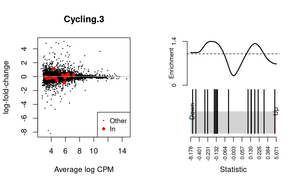
Cycling.3

Show code

n <- "Cycling.3"
md <- metadata(de_results[[n]])
y <- md$y
y_design <- md$design
y_index <- ids2indices(
  list(`BCL2-family` = bcl2_df$Approved.symbol),
  rownames(y))
fry(
  y,
  index = y_index,
  design = y_design,
  coef = "TreatmentInfected") %>%
  knitr::kable(
    caption = "Results of applying `fry()` to the RNA-seq differential expression results using the supplied gene sets. A significant 'Up' P-value means that the differential expression results found in the RNA-seq data are positively correlated with the expression signature from the corresponding gene set. Conversely, a significant 'Down' P-value means that the differential expression log-fold-changes are negatively correlated with the expression signature from the corresponding gene set. A significant 'Mixed' P-value means that the genes in the set tend to be differentially expressed without regard for direction.")

Table 11: Results of applying fry() to the RNA-seq differential expression results using the supplied gene sets. A significant ‘Up’ P-value means that the differential expression results found in the RNA-seq data are positively correlated with the expression signature from the corresponding gene set. Conversely, a significant ‘Down’ P-value means that the differential expression log-fold-changes are negatively correlated with the expression signature from the corresponding gene set. A significant ‘Mixed’ P-value means that the genes in the set tend to be differentially expressed without regard for direction.

	NGenes	Direction	PValue	PValue.Mixed
BCL2-family	16	Down	0.8767046	0.102535

Show code

dgelrt <- glmTreat(md$fit, coef = "TreatmentInfected", lfc = log2(1.5))
par(mfrow = c(1, 2))
y_status <- rep("Other", nrow(dgelrt))
y_status[rownames(dgelrt) %in% bcl2_df$Approved.symbol] <- "In"
plotMD(
  dgelrt,
  status = y_status,
  values = "In",
  hl.col = "red",
  legend = "bottomright",
  main = n)
abline(h = 0, col = "darkgrey")
barcodeplot(
  statistics = dgelrt$table$logFC,
  index = rownames(dgelrt) %in% bcl2_df$Approved.symbol)

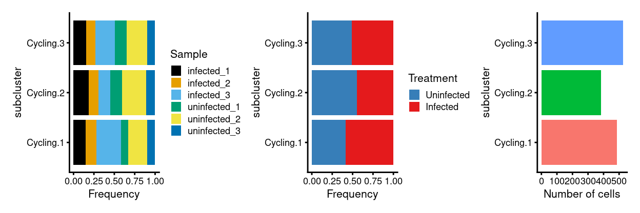
DA

• Number of cells/label/sample

Show code

abundances <- table(x$subcluster, x$Sample)
abundances <- unclass(abundances)
abundances

            infected_1 infected_2 infected_3 uninfected_1
  Cycling.1         73         65        147           42
  Cycling.2         72         45         55           55
  Cycling.3         81         61        125           74

            uninfected_2 uninfected_3
  Cycling.1          112           48
  Cycling.2          113           43
  Cycling.3          133           51

Show code

p1 <- plotUMAP(
  x,
  colour_by = "subcluster",
  text_by = "subcluster",
  point_size = 0.5,
  point_alpha = 1,
  text_size = 4)
p2 <- plotUMAP(
  x,
  colour_by = "Treatment",
  point_size = 0.5,
  point_alpha = 1) +
  scale_colour_manual(values = treatment_colours)
p1 + p2

Show code

p3 <- ggplot(as.data.frame(colData(x)[, c("subcluster", "Sample")])) +
  geom_bar(
    aes(x = subcluster, fill = Sample),
    position = position_fill(reverse = TRUE)) +
  coord_flip() +
  ylab("Frequency") +
  scale_fill_manual(values = sample_colours) +
  theme_cowplot(font_size = 8)
p4 <- ggplot(as.data.frame(colData(x)[, c("subcluster", "Treatment")])) +
  geom_bar(
    aes(x = subcluster, fill = Treatment),
    position = position_fill(reverse = TRUE)) +
  coord_flip() +
  ylab("Frequency") +
  scale_fill_manual(values = treatment_colours) +
  theme_cowplot(font_size = 8)
p5 <- ggplot(as.data.frame(colData(x)[, "subcluster", drop = FALSE])) +
  geom_bar(aes(x = subcluster, fill = subcluster)) +
  coord_flip() +
  ylab("Number of cells") +
  theme_cowplot(font_size = 8) +
  guides(fill = FALSE)
p3 + p4 + p5 + plot_layout(ncol = 3)

• TRUE/FALSE if label can be tested for DA

Show code

extra.info <- colData(sce)[match(colnames(abundances), sce$Sample), ]
y.ab <- DGEList(abundances, samples = extra.info)

keep <- filterByExpr(y.ab, group = y.ab$samples$Treatment)
keep

Cycling.1 Cycling.2 Cycling.3
     TRUE      TRUE      TRUE 

• Number of labels that are DA (-1 means less abundant in Infected vs. Uninfected, 0 means not DE, 1 means more abundant in Infected vs. Uninfected)

Show code

y.ab <- y.ab[keep,]

design <- model.matrix(~Treatment, y.ab$samples)

y.ab <- estimateDisp(y.ab, design, trend = "none")
fit.ab <- glmFit(y.ab)
res <- glmLRT(fit.ab, coef = "TreatmentInfected")
summary(decideTests(res))

       TreatmentInfected
Down                   0
NotSig                 3
Up                     0

• Full results (negative logFC means less abundant in Infected vs. Uninfected, positive logFC means more abundant in Infected vs. Uninfected)

Show code

topTags(res, n = Inf)

Coefficient:  TreatmentInfected
                logFC   logCPM        LR     PValue       FDR
Cycling.1  0.37294181 18.40769 3.7213695 0.05372029 0.1611609
Cycling.2 -0.35382545 18.10346 2.1597911 0.14166395 0.2124959
Cycling.3 -0.06526804 18.53074 0.2197015 0.63926749 0.6392675

Concluding remarks

Show code

saveRDS(
  sce.ignoring_cycling_subset,
  here("data", "SCEs", "C057_Cooney.ignoring_cycling_subset.sce.rds"),
  compress = "xz")
saveRDS(
  sce.cycling_subset_Sample,
  here("data", "SCEs", "C057_Cooney.cycling_subset_Sample.sce.rds"),
  compress = "xz")
saveRDS(
  not_cycling_sce.subcluster_Sample,
  here("data", "SCEs", "C057_Cooney.not_cycling.subcluster_Sample.sce.rds"),
  compress = "xz")
saveRDS(
  cycling_sce.subcluster_Sample,
  here("data", "SCEs", "C057_Cooney.cycling.subcluster_Sample.sce.rds"),
  compress = "xz")

The aggregated SummarizedExperiment objects are available (see data/SCEs/C057_Cooney.ignoring_cycling_subset.sce.rds, data/SCEs/C057_Cooney.cycling_subset_Sample.sce.rds, data/SCEs/C057_Cooney.not_cycling.subcluster_Sample.sce.rds, and data/SCEs/C057_Cooney.cycling.subcluster_Sample.sce.rds). These can be used for visualizations with iSEE.

The output/DEGs/ directory contains CSV files summarising the differential expression results and PDFs showing the pseudobulk expression data for each DEG.

Additional information

The following are available on request:

• Full CSV tables of any data presented.
• PDF/PNG files of any static plots.

Session info

The analysis and this document were prepared using the following software (click triangle to expand)

Show code

sessioninfo::session_info()

─ Session info ─────────────────────────────────────────────────────
 setting  value
 version  R version 4.0.3 (2020-10-10)
 os       CentOS Linux 7 (Core)
 system   x86_64, linux-gnu
 ui       X11
 language (EN)
 collate  en_US.UTF-8
 ctype    en_US.UTF-8
 tz       Australia/Melbourne
 date     2021-12-03

─ Packages ─────────────────────────────────────────────────────────
 ! package              * version  date       lib
 P annotate               1.68.0   2020-10-27 [?]
 P AnnotationDbi          1.52.0   2020-10-27 [?]
 P assertthat             0.2.1    2019-03-21 [?]
 P beachmat               2.6.4    2020-12-20 [?]
 P beeswarm               0.2.3    2016-04-25 [?]
 P Biobase              * 2.50.0   2020-10-27 [?]
   BiocGenerics         * 0.36.0   2020-10-27 [1]
 P BiocManager            1.30.10  2019-11-16 [?]
 P BiocNeighbors          1.8.2    2020-12-07 [?]
   BiocParallel           1.24.1   2020-11-06 [1]
 P BiocSingular           1.6.0    2020-10-27 [?]
   BiocStyle              2.18.1   2020-11-24 [1]
 P bit                    4.0.4    2020-08-04 [?]
 P bit64                  4.0.5    2020-08-30 [?]
 P bitops                 1.0-6    2013-08-17 [?]
 P blob                   1.2.1    2020-01-20 [?]
 P bluster                1.0.0    2020-10-27 [?]
 P bslib                  0.2.4    2021-01-25 [?]
 P cachem                 1.0.4    2021-02-13 [?]
 P cli                    2.3.1    2021-02-23 [?]
 P colorspace             2.0-0    2020-11-11 [?]
 P cowplot              * 1.1.1    2020-12-30 [?]
 P crayon                 1.4.1    2021-02-08 [?]
 P DBI                    1.1.1    2021-01-15 [?]
 P DelayedArray           0.16.2   2021-02-26 [?]
 P DelayedMatrixStats     1.12.3   2021-02-03 [?]
 P DESeq2                 1.30.1   2021-02-19 [?]
 P digest                 0.6.27   2020-10-24 [?]
 P distill                1.2      2021-01-13 [?]
 P downlit                0.2.1    2020-11-04 [?]
 P dplyr                  1.0.4    2021-02-02 [?]
 P dqrng                  0.2.1    2019-05-17 [?]
 P edgeR                * 3.32.1   2021-01-14 [?]
 P ellipsis               0.3.1    2020-05-15 [?]
 P evaluate               0.14     2019-05-28 [?]
 P fansi                  0.4.2    2021-01-15 [?]
 P farver                 2.1.0    2021-02-28 [?]
 P fastmap                1.1.0    2021-01-25 [?]
 P genefilter             1.72.1   2021-01-21 [?]
 P geneplotter            1.68.0   2020-10-27 [?]
 P generics               0.1.0    2020-10-31 [?]
 P GenomeInfoDb         * 1.26.2   2020-12-08 [?]
   GenomeInfoDbData       1.2.4    2021-02-04 [1]
 P GenomicRanges        * 1.42.0   2020-10-27 [?]
 P ggbeeswarm             0.6.0    2017-08-07 [?]
 P ggplot2              * 3.3.3    2020-12-30 [?]
 P Glimma                 2.0.0    2020-10-27 [?]
 P glue                   1.4.2    2020-08-27 [?]
 P gridExtra              2.3      2017-09-09 [?]
 P gtable                 0.3.0    2019-03-25 [?]
 P here                 * 1.0.1    2020-12-13 [?]
 P highr                  0.8      2019-03-20 [?]
 P htmltools              0.5.1.1  2021-01-22 [?]
 P htmlwidgets            1.5.3    2020-12-10 [?]
 P httr                   1.4.2    2020-07-20 [?]
 P igraph                 1.2.6    2020-10-06 [?]
 P IRanges              * 2.24.1   2020-12-12 [?]
 P irlba                  2.3.3    2019-02-05 [?]
 P jquerylib              0.1.3    2020-12-17 [?]
 P jsonlite               1.7.2    2020-12-09 [?]
 P knitr                  1.31     2021-01-27 [?]
 P labeling               0.4.2    2020-10-20 [?]
 P lattice                0.20-41  2020-04-02 [?]
 P lifecycle              1.0.0    2021-02-15 [?]
   limma                * 3.46.0   2020-10-27 [1]
 P locfit                 1.5-9.4  2020-03-25 [?]
 P magrittr             * 2.0.1    2020-11-17 [?]
 P Matrix                 1.3-2    2021-01-06 [?]
   MatrixGenerics       * 1.2.1    2021-01-30 [1]
 P matrixStats          * 0.58.0   2021-01-29 [?]
 P memoise                2.0.0    2021-01-26 [?]
 P munsell                0.5.0    2018-06-12 [?]
 P patchwork            * 1.1.1    2020-12-17 [?]
 P pheatmap               1.0.12   2019-01-04 [?]
 P pillar                 1.5.0    2021-02-22 [?]
 P pkgconfig              2.0.3    2019-09-22 [?]
 P purrr                  0.3.4    2020-04-17 [?]
 P R6                     2.5.0    2020-10-28 [?]
 P RColorBrewer           1.1-2    2014-12-07 [?]
 P Rcpp                   1.0.6    2021-01-15 [?]
 P RCurl                  1.98-1.2 2020-04-18 [?]
 P rlang                  0.4.10   2020-12-30 [?]
 P rmarkdown              2.11     2021-09-14 [?]
 P rprojroot              2.0.2    2020-11-15 [?]
 P RSQLite                2.2.3    2021-01-24 [?]
 P rsvd                   1.0.3    2020-02-17 [?]
 P S4Vectors            * 0.28.1   2020-12-09 [?]
 P sass                   0.3.1    2021-01-24 [?]
 P scales                 1.1.1    2020-05-11 [?]
 P scater               * 1.18.6   2021-02-26 [?]
 P scran                * 1.18.5   2021-02-04 [?]
 P scuttle                1.0.4    2020-12-17 [?]
 P sessioninfo            1.1.1    2018-11-05 [?]
 P SingleCellExperiment * 1.12.0   2020-10-27 [?]
 P sparseMatrixStats      1.2.1    2021-02-02 [?]
 P statmod                1.4.35   2020-10-19 [?]
 P stringi                1.5.3    2020-09-09 [?]
 P stringr                1.4.0    2019-02-10 [?]
 P SummarizedExperiment * 1.20.0   2020-10-27 [?]
 P survival               3.2-7    2020-09-28 [?]
 P tibble                 3.1.0    2021-02-25 [?]
 P tidyselect             1.1.0    2020-05-11 [?]
 P utf8                   1.1.4    2018-05-24 [?]
 P vctrs                  0.3.6    2020-12-17 [?]
 P vipor                  0.4.5    2017-03-22 [?]
 P viridis                0.5.1    2018-03-29 [?]
 P viridisLite            0.3.0    2018-02-01 [?]
 P withr                  2.4.1    2021-01-26 [?]
 P xaringanExtra          0.5.5    2021-12-03 [?]
 P xfun                   0.28     2021-11-04 [?]
 P XML                    3.99-0.5 2020-07-23 [?]
 P xtable                 1.8-4    2019-04-21 [?]
 P XVector                0.30.0   2020-10-27 [?]
 P yaml                   2.2.1    2020-02-01 [?]
 P zlibbioc               1.36.0   2020-10-27 [?]
 source
 Bioconductor
 Bioconductor
 CRAN (R 4.0.0)
 Bioconductor
 CRAN (R 4.0.0)
 Bioconductor
 Bioconductor
 CRAN (R 4.0.0)
 Bioconductor
 Bioconductor
 Bioconductor
 Bioconductor
 CRAN (R 4.0.0)
 CRAN (R 4.0.0)
 CRAN (R 4.0.0)
 CRAN (R 4.0.0)
 Bioconductor
 CRAN (R 4.0.3)
 CRAN (R 4.0.3)
 CRAN (R 4.0.3)
 CRAN (R 4.0.3)
 CRAN (R 4.0.3)
 CRAN (R 4.0.3)
 CRAN (R 4.0.3)
 Bioconductor
 Bioconductor
 Bioconductor
 CRAN (R 4.0.2)
 CRAN (R 4.0.3)
 CRAN (R 4.0.3)
 CRAN (R 4.0.3)
 CRAN (R 4.0.0)
 Bioconductor
 CRAN (R 4.0.0)
 CRAN (R 4.0.0)
 CRAN (R 4.0.3)
 CRAN (R 4.0.3)
 CRAN (R 4.0.3)
 Bioconductor
 Bioconductor
 CRAN (R 4.0.3)
 Bioconductor
 Bioconductor
 Bioconductor
 CRAN (R 4.0.0)
 CRAN (R 4.0.3)
 Bioconductor
 CRAN (R 4.0.0)
 CRAN (R 4.0.0)
 CRAN (R 4.0.0)
 CRAN (R 4.0.3)
 CRAN (R 4.0.0)
 CRAN (R 4.0.3)
 CRAN (R 4.0.3)
 CRAN (R 4.0.0)
 CRAN (R 4.0.2)
 Bioconductor
 CRAN (R 4.0.0)
 CRAN (R 4.0.3)
 CRAN (R 4.0.3)
 CRAN (R 4.0.3)
 CRAN (R 4.0.0)
 CRAN (R 4.0.0)
 CRAN (R 4.0.3)
 Bioconductor
 CRAN (R 4.0.0)
 CRAN (R 4.0.3)
 CRAN (R 4.0.3)
 Bioconductor
 CRAN (R 4.0.3)
 CRAN (R 4.0.3)
 CRAN (R 4.0.0)
 CRAN (R 4.0.3)
 CRAN (R 4.0.0)
 CRAN (R 4.0.3)
 CRAN (R 4.0.0)
 CRAN (R 4.0.0)
 CRAN (R 4.0.2)
 CRAN (R 4.0.0)
 CRAN (R 4.0.3)
 CRAN (R 4.0.0)
 CRAN (R 4.0.3)
 CRAN (R 4.0.0)
 CRAN (R 4.0.3)
 CRAN (R 4.0.3)
 CRAN (R 4.0.0)
 Bioconductor
 CRAN (R 4.0.3)
 CRAN (R 4.0.0)
 Bioconductor
 Bioconductor
 Bioconductor
 CRAN (R 4.0.0)
 Bioconductor
 Bioconductor
 CRAN (R 4.0.2)
 CRAN (R 4.0.0)
 CRAN (R 4.0.0)
 Bioconductor
 CRAN (R 4.0.2)
 CRAN (R 4.0.3)
 CRAN (R 4.0.0)
 CRAN (R 4.0.0)
 CRAN (R 4.0.3)
 CRAN (R 4.0.0)
 CRAN (R 4.0.0)
 CRAN (R 4.0.0)
 CRAN (R 4.0.3)
 Github (gadenbuie/xaringanExtra@cc1f613)
 CRAN (R 4.0.3)
 CRAN (R 4.0.0)
 CRAN (R 4.0.0)
 Bioconductor
 CRAN (R 4.0.0)
 Bioconductor

[1] /stornext/Projects/score/Analyses/C057_Cooney/renv/library/R-4.0/x86_64-pc-linux-gnu
[2] /tmp/RtmpyCwH1Q/renv-system-library
[3] /stornext/System/data/apps/R/R-4.0.3/lib64/R/library

 P ── Loaded and on-disk path mismatch.