Show code
library(here)
library(magrittr)
library(BiocStyle)
library(dplyr)
library(janitor)
library(cowplot)

source(here("code", "helper_functions.R"))

# NOTE: Using >= 4 cores seizes up my laptop. Can use more on unix box.
options("mc.cores" = ifelse(Sys.info()[["nodename"]] == "PC1331", 2L, 3L))

knitr::opts_chunk$set(fig.path = "C057_Cooney.demultiplex_files/")
Introduction
Cells were obtained from six samples. These samples were processed a technique called using Cell Hashing, a method that enables sample multiplexing. Cell Hashing uses a series of oligo-tagged antibodies against ubiquitously expressed surface proteins with different barcodes to uniquely label cells from distinct samples, which can be subsequently pooled in one scRNA-seq run. By sequencing these tags alongside the cellular transcriptome, we can assign each cell to its sample of origin, and robustly identify doublets originating from multiple samples.
In a typical Cell Hashing experiment, each sample is uniquely labelled with a single hashtag oligonucleotide (HTO). However, in this experiment we needed to label 6 samples but only had 5 HTOs. We decided to uniquely label five of the samples (three infected, two uninfected) with a single HTO and to label the sixth sample with all five HTOs. This non-standard use of HTOs meant we could not rely on standard cell hashing demultiplexing routines, like that available in Seurat.
Setting up the data
The count data were processed using CellRanger and the DropletUtils R/Bioconductor packages. The counts and their metadata are available in a SingleCellExperiment object available as data/SCEs/HTLV_GEX_HTO.CellRanger.SCE.rds. These are the unfiltered data, i.e. the data includes all potential genes and barcodes.
Calling cells from empty droplets
An interesting aspect of droplet-based data is that we have no prior knowledge about which droplets (i.e. cell barcodes) actually contain cells, and which are empty. Thus, we need to call cells from empty droplets based on the observed expression profiles. This is done separately for each 10x run.
Calling empty droplets is not entirely straightforward as empty droplets can contain ambient (i.e. extracellular) RNA that can be captured and sequenced. The distribution of total counts exhibits a sharp transition between barcodes with large and small total counts (Figure 1), probably corresponding to cell-containing and empty droplets respectively.
Show code
library(DropletUtils)
bcrank <- barcodeRanks(counts(sce))
# Only showing unique points for plotting speed.
uniq <- !duplicated(bcrank$rank)
plot(
  x = bcrank$rank[uniq],
  y = bcrank$total[uniq],
  log = "xy",
  xlab = "Rank",
  ylab = "Total UMI count",
  main = "C057_Cooney",
  cex.lab = 1.2,
  xlim = c(1, 500000),
  ylim = c(1, 50000))
abline(h = metadata(bcrank)$inflection, col = "darkgreen", lty = 2)
abline(h = metadata(bcrank)$knee, col = "dodgerblue", lty = 2)
legend(
  "bottomleft",
  legend = c("Inflection", "Knee"),
  col = c("darkgreen", "dodgerblue"),
  lty = 2,
  cex = 1.2)
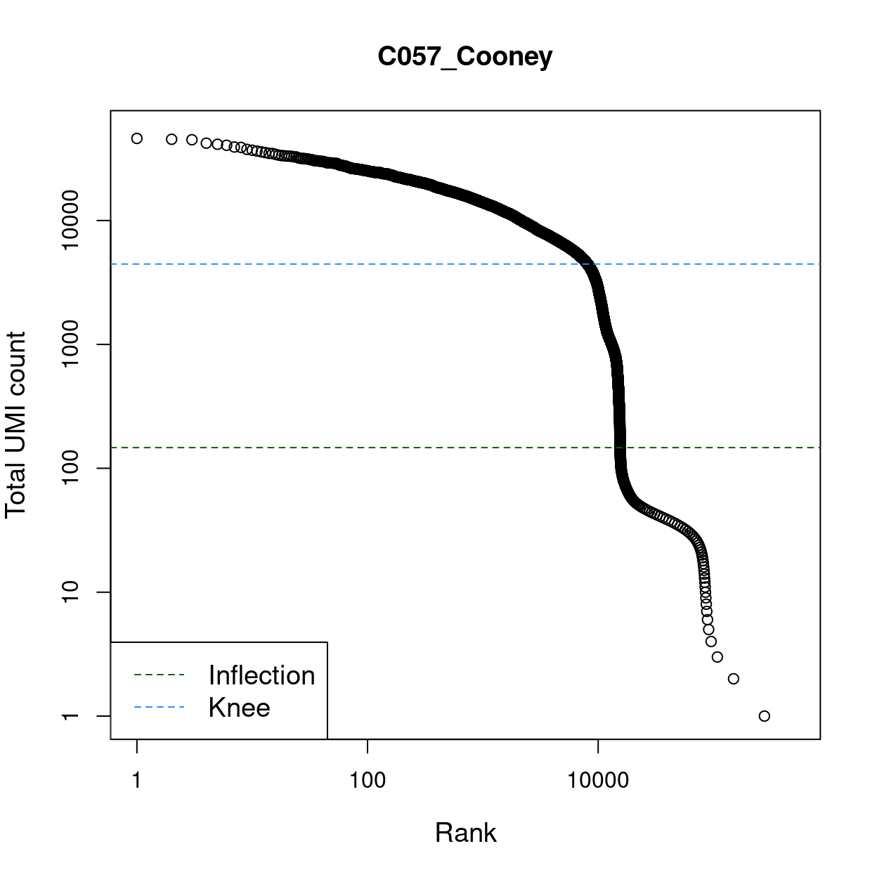
Figure 1: Total UMI count for each barcode in the dataset, plotted against its rank (in decreasing order of total counts). The inferred locations of the inflection (dark green dashed lines) and knee points (blue dashed lines) are also shown.
We use the emptyDrops() function from the DropletUtils package to test whether the expression profile for each cell barcode is significantly different from the ambient RNA pool (Lun et al. 2018). This tends to be less conservative than the cell calling algorithm from the CellRanger pipeline, which often discards genuine cells with low RNA content (and thus low total counts). Any significant deviation indicates that the barcode corresponds to a cell-containing droplet. We call cells at a false discovery rate (FDR) of 0.1%, meaning that no more than 0.1% of our called barcodes should be empty droplets on average.
Show code
empties <- readRDS(
  here("data", "emptyDrops", "C057_Cooney.emptyDrops.rds"))
mutate(as.data.frame(empties), Sample = rep("C057", nrow(empties))) %>%
  group_by(Sample) %>%
  summarise(
    keep = sum(FDR <= 0.001, na.rm = TRUE),
    n = n(),
    remove = n - keep) %>%
  mutate(library = factor(Sample)) %>%
  select(library, keep, remove) %>%
  knitr::kable(
    caption = "Number of droplets kept and removed after filtering empty drops.")
| library | keep | remove |
|---|---|---|
| C057 | 13944 | 723336 |
Demultiplexing with hashtag oligos (HTOs)
Motivation
James provided me with a table linking HTOs to samples, shown below.
Show code
hto_to_sample_df <- data.frame(
  HTO = c(paste0("human_", 1:5), "human_1-human_2-human_3-human_4-human_5"),
  Sample = c(paste0("infected_", 1:3), paste0("uninfected_", 1:3)),
  Treatment = c(rep("Infected", 3), rep("Uninfected", 3)),
  Replicate = rep(1:3, 2))

knitr::kable(hto_to_sample_df, caption = "Table linking HTOs to samples")
| HTO | Sample | Treatment | Replicate |
|---|---|---|---|
| human_1 | infected_1 | Infected | 1 |
| human_2 | infected_2 | Infected | 2 |
| human_3 | infected_3 | Infected | 3 |
| human_4 | uninfected_1 | Uninfected | 1 |
| human_5 | uninfected_2 | Uninfected | 2 |
| human_1-human_2-human_3-human_4-human_5 | uninfected_3 | Uninfected | 3 |
Analysis
We only use the droplets identified as non-empty in Calling cells from empty droplets.
These samples were processed using 5 HTOs (human_1, human_2, human_3, human_4, and human_5). Nonetheless, we ran CellRanger using a larger panel of HTOs (n = 38) to enable us to check for background contamination of HTOs.
Figure 2 plots the distribution of each HTO counts for the the 8 most frequently HTOs detected and shows that HTOs human_1, human_2, human_3, human_4, and human_5 are clearly detected more frequently than the other barcodes, as we would hope.
Show code
par(mfrow = c(2, 4))
o <- order(rowSums(counts(altExp(sce, "Antibody Capture"))), decreasing = TRUE)
for (i in o[1:8]) {
  if (rowSums(counts(altExp(sce, "Antibody Capture")))[i] > 10) {
    plot(
      table(counts(altExp(sce, "Antibody Capture"))[i, ]),
      main = rownames(altExp(sce, "Antibody Capture"))[i],
      xlim = c(1, 10 ^ 5),
      log = "x",
      xlab = "Detections",
      ylab = "Frequency")
    abline(v = 10, col = "red")
  }
}
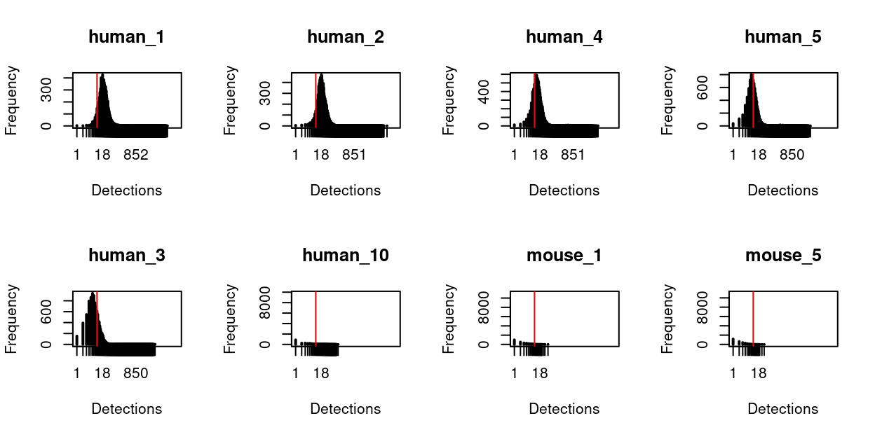
Figure 2: Distribution of HTO counts in the dataset. Only those HTOs with more detected in at least one cell are shown. The red vertical line denotes detecting the HTO 10 times in a sample.
We therefore focus on assigning cells to just the human_1, human_2, human_3, human_4, and human_5 HTOs, along with the combination of all five HTOs.
Show code
altExp(sce, "Antibody Capture") <- altExp(
  sce, "Antibody Capture")[paste0("human_", 1:5), ]

sce$hto_sum <- colSums(counts(altExp(sce)))
ambient <- rowMeans(counts(altExp(sce_empties)))[rownames(altExp(sce))]

hto_low_counts_cutoff <- metadata(
  barcodeRanks(counts(altExp(sce_empties))))$inflection
To do so, we will cluster the (log normalized) HTO expression profiles and manually annotate the resulting clusters. We perform median-based size normalization of the HTO count data.1. This requires an estimate of the ambient expression of each HTO, which we estimate from the empty droplets.
Show code
as.data.frame(ambient) %>%
  knitr::kable(digits = 1, caption = "Estimated ambient counts for each HTO.")
| ambient | |
|---|---|
| human_1 | 4.3 |
| human_2 | 3.1 |
| human_3 | 0.9 |
| human_4 | 1.8 |
| human_5 | 1.2 |
Show code
library(scater)
sf_amb <- medianSizeFactors(
  altExp(sce, "Antibody Capture"),
  reference = ambient)
# NOTE: Size factors should be positive.
sf_amb[sf_amb == 0] <- min(sf_amb[sf_amb > 0])
sizeFactors(altExp(sce, "Antibody Capture")) <- sf_amb
altExp(sce, "Antibody Capture") <- logNormCounts(
  altExp(sce, "Antibody Capture"))
We then apply graph-based clustering to the normalized log-expression of the HTOs to identify samples with similar HTO expression profiles. We deliberately overcluster the data in order to obtain quite specific clusters.
Show code
library(scran)
# NOTE: `d = NA` means no dimensionality reduction is performed.
# NOTE: `k = 5` was selected by trial and error.
g <- buildSNNGraph(altExp(sce, "Antibody Capture"), k = 5, d = NA)
clusters <- igraph::cluster_louvain(g)$membership
# NOTE: Orders cluster labels (1, ..., N) so that the biggest cluster is N and
#       the smallest is 1.
sce$hto_cluster <- factor(
  as.integer(factor(clusters, names(sort(table(clusters), decreasing = TRUE)))))
hto_cluster_colours <- setNames(
  Polychrome::glasbey.colors(nlevels(sce$hto_cluster) + 1)[-1],
  levels(sce$hto_cluster))
sce$hto_cluster_colours <- hto_cluster_colours[sce$hto_cluster]
Figure 3 is a heatmap of the counts for each HTO in each droplet. We can clearly see droplets corresponding to singlets from each of the six samples, i.e. those droplets with large counts for exactly one of the human_1, human_2, human_3, human_4, or human_5 HTOs and droplets with large counts for all five HTOs.
Show code
library(pheatmap)
pheatmap(
  log2(counts(altExp(sce)) + 1)[
    , order(sce$hto_cluster, sce$hto_sum, decreasing = c(FALSE, TRUE))],
  color = viridisLite::inferno(100),
  cluster_rows = FALSE,
  cluster_cols = FALSE,
  annotation_col = data.frame(
    hto_cluster = sce$hto_cluster,
    sum = log10(sce$hto_sum),
    low = ifelse(sce$hto_sum < hto_low_counts_cutoff, "Low", "High"),
    row.names = colnames(sce)),
  annotation_row = data.frame(ambient = log10(ambient)),
  annotation_colors = list(
    hto_cluster = hto_cluster_colours,
    sum = viridisLite::viridis(101),
    low = c("Low" = "red", "High" = "white"),
    ambient = viridisLite::viridis(101)),
  show_colnames = FALSE,
  scale = "none",
  fontsize = 6)
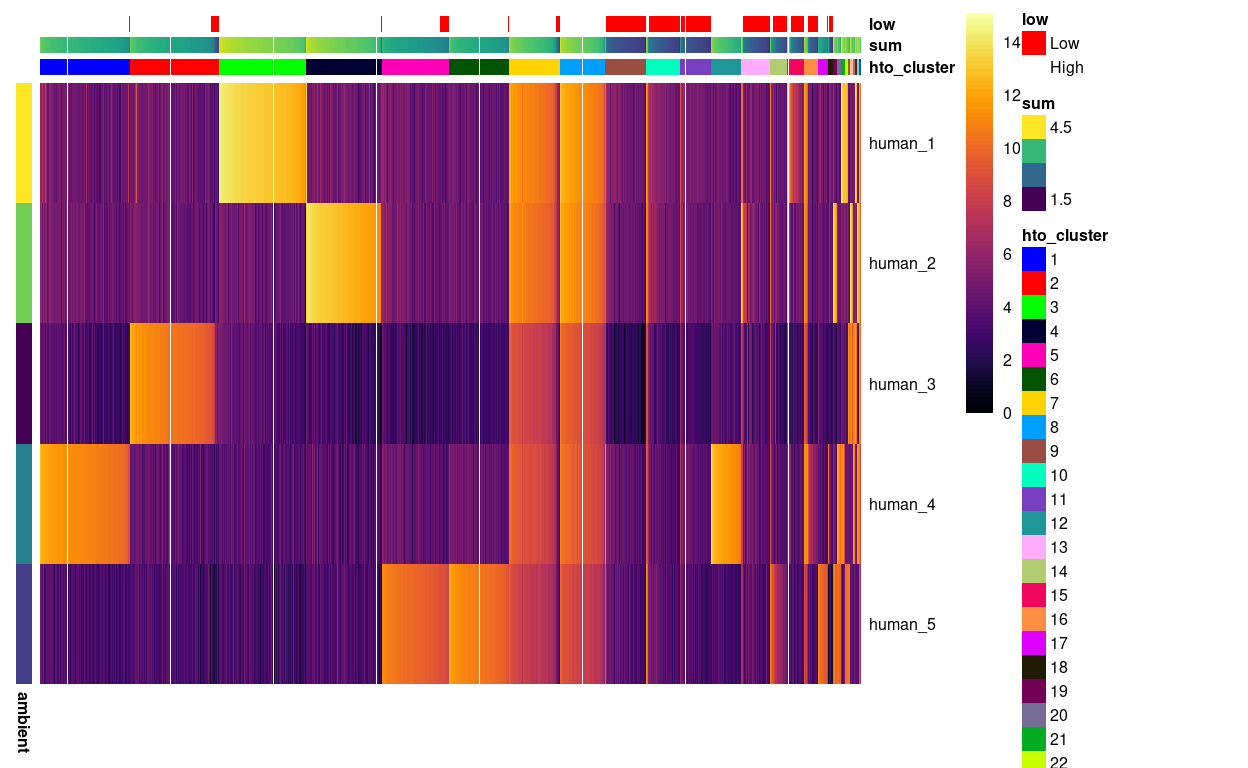
Figure 3: Heatmap of HTO log2(counts + 1) for the droplets. Columns are ordered by cluster and then HTO library size. Each droplet (column) is annotated by the (log10) HTO library size (sum) and whether that is smaller than the a cutoff estimated from the empty droplets. Each HTO (row) is annotated by the (log10) average count of the HTO in the empty droplets (ambient).
On the basis of Figure 3, we assign these singlets to their sample of origin:
Show code
singlet_clusters <- as.character(c(1:8, 12))
singlet_cluster_to_hto_tbl <- tibble::tribble(
  ~hto_cluster, ~HTO,
  "1",          "human_4",
  "2",          "human_3",
  "3",          "human_1",
  "4",          "human_2",
  "5",          "human_5",
  "6",          "human_5",
  "7",          "human_1-human_2-human_3-human_4-human_5",
  "8",          "human_1-human_2-human_3-human_4-human_5",
  "12",         "human_4")
stopifnot(identical(singlet_clusters, singlet_cluster_to_hto_tbl$hto_cluster))

left_join(singlet_cluster_to_hto_tbl, hto_to_sample_df) %>%
  knitr::kable(., caption = "Assignments of singlet clusters to samples.")
| hto_cluster | HTO | Sample | Treatment | Replicate |
|---|---|---|---|---|
| 1 | human_4 | uninfected_1 | Uninfected | 1 |
| 2 | human_3 | infected_3 | Infected | 3 |
| 3 | human_1 | infected_1 | Infected | 1 |
| 4 | human_2 | infected_2 | Infected | 2 |
| 5 | human_5 | uninfected_2 | Uninfected | 2 |
| 6 | human_5 | uninfected_2 | Uninfected | 2 |
| 7 | human_1-human_2-human_3-human_4-human_5 | uninfected_3 | Uninfected | 3 |
| 8 | human_1-human_2-human_3-human_4-human_5 | uninfected_3 | Uninfected | 3 |
| 12 | human_4 | uninfected_1 | Uninfected | 1 |
We then turn our attention to the remaining clusters. Figure 4 shows that the largest remaining clusters contain droplets with ‘low’ library sizes, which are hard to confidently assign to a sample.
Show code
tmp_sce <- sce[, !sce$hto_cluster %in% singlet_clusters]
pheatmap(
  log2(counts(altExp(tmp_sce)) + 1)[
    , order(tmp_sce$hto_cluster, tmp_sce$hto_sum, decreasing = c(FALSE, TRUE))],
  color = viridisLite::inferno(100),
  cluster_rows = FALSE,
  cluster_cols = FALSE,
  annotation_col = data.frame(
    hto_cluster = sce$hto_cluster,
    sum = log10(sce$hto_sum),
    low = ifelse(sce$hto_sum < hto_low_counts_cutoff, "Low", "High"),
    row.names = colnames(sce)),
  annotation_row = data.frame(ambient = log10(ambient)),
  annotation_colors = list(
    # NOTE: Select 'active' colour levels.
    hto_cluster = hto_cluster_colours[
      levels(factor(tmp_sce$hto_cluster))],
    sum = viridisLite::viridis(101),
    low = c("Low" = "red", "High" = "white"),
    ambient = viridisLite::viridis(101)),
  show_colnames = FALSE,
  scale = "none",
  fontsize = 6)
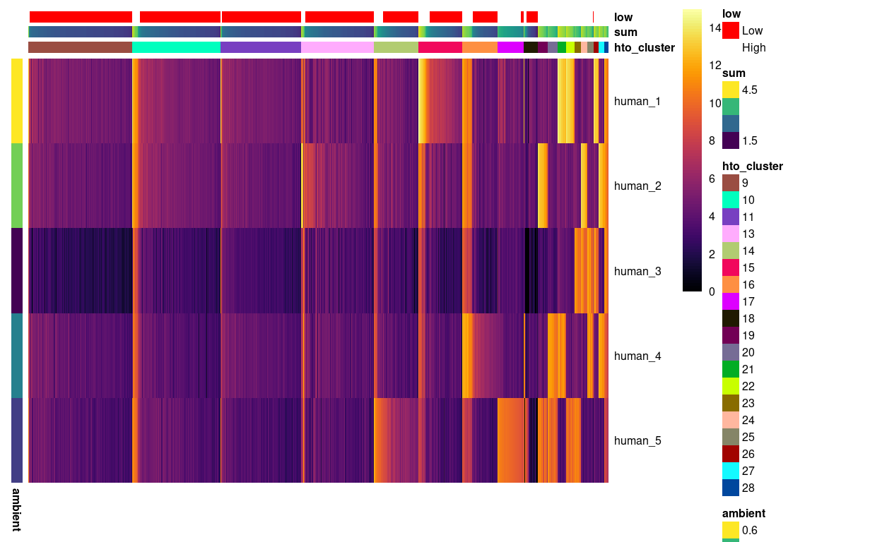
Figure 4: Heatmap of HTO log2(counts + 1) for the droplets not yet assigned to a sample of origin. Columns are ordered by cluster and then HTO library size. Each droplet (column) is annotated by the (log10) HTO library size (sum) and whether that is smaller than the a cutoff estimated from the empty droplets. Each HTO (row) is annotated by the (log10) average count of the HTO in the empty droplets (ambient).
On the basis of Figure 4, we opt for a conservative approach that labels droplets in the these clusters as ambiguous (i.e. we cannot confidently assign them to a sample of origin).
Show code
ambiguous_clusters <- as.character(c(9:11, 13:16, 18))
ambiguous_cluster_to_hto_tbl <- tibble::tribble(
    ~hto_cluster, ~HTO,
    "9",          "ambiguous",
    "10",          "ambiguous",
    "11",         "ambiguous",
    "13",         "ambiguous",
    "14",         "ambiguous",
    "15",         "ambiguous",
    "16",         "ambiguous",
    "18",         "ambiguous")
stopifnot(
  identical(ambiguous_clusters, ambiguous_cluster_to_hto_tbl$hto_cluster))

left_join(ambiguous_cluster_to_hto_tbl, hto_to_sample_df) %>%
  knitr::kable(., caption = "Clusters containing `ambiguous` droplets.")
| hto_cluster | HTO | Sample | Treatment | Replicate |
|---|---|---|---|---|
| 9 | ambiguous | NA | NA | NA |
| 10 | ambiguous | NA | NA | NA |
| 11 | ambiguous | NA | NA | NA |
| 13 | ambiguous | NA | NA | NA |
| 14 | ambiguous | NA | NA | NA |
| 15 | ambiguous | NA | NA | NA |
| 16 | ambiguous | NA | NA | NA |
| 18 | ambiguous | NA | NA | NA |
We then turn our attention to the remaining clusters. Figure 5 shows that the remaining clusters largely contain droplets with 2 HTOs, which correspond to droplets containing two cells (‘doublets’), a cluster that appears to be droplets with the human-5 HTO, and a small cluster of droplets that appear to contain all five HTOs.
Show code
tmp_sce <- sce[, !sce$hto_cluster %in% c(singlet_clusters, ambiguous_clusters)]
pheatmap(
  log2(counts(altExp(tmp_sce)) + 1)[
    , order(tmp_sce$hto_cluster, tmp_sce$hto_sum, decreasing = c(FALSE, TRUE))],
  color = viridisLite::inferno(100),
  cluster_rows = FALSE,
  cluster_cols = FALSE,
  annotation_col = data.frame(
    hto_cluster = sce$hto_cluster,
    sum = log10(sce$hto_sum),
    low = ifelse(sce$hto_sum < hto_low_counts_cutoff, "Low", "High"),
    row.names = colnames(sce)),
  annotation_row = data.frame(ambient = log10(ambient)),
  annotation_colors = list(
    # NOTE: Select 'active' colour levels.
    hto_cluster = hto_cluster_colours[
      levels(factor(tmp_sce$hto_cluster))],
    sum = viridisLite::viridis(101),
    low = c("Low" = "red", "High" = "white"),
    ambient = viridisLite::viridis(101)),
  show_colnames = FALSE,
  scale = "none",
  fontsize = 6)
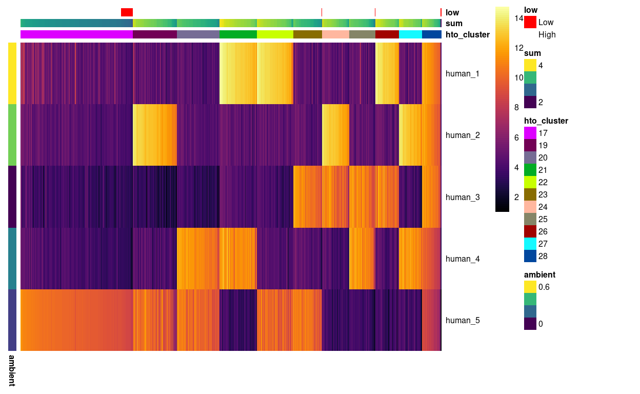
Figure 5: Heatmap of HTO log2(counts + 1) for the droplets not yet assigned to a sample of origin. Columns are ordered by cluster and then HTO library size. Each droplet (column) is annotated by the (log10) HTO library size (sum) and whether that is smaller than the a cutoff estimated from the empty droplets. Each HTO (row) is annotated by the (log10) average count of the HTO in the empty droplets (ambient).
On the basis of Figure 5, we assign droplets in these clusters accordingly:
Show code
mostly_doublet_clusters <- as.character(c(17, 19:28))
mostly_doublet_cluster_to_hto_tbl <- tibble::tribble(
    ~hto_cluster,  ~HTO,
    "17",          "human_5",
    "19",          "doublet",
    "20",          "doublet",
    "21",          "doublet",
    "22",          "doublet",
    "23",          "doublet",
    "24",          "doublet",
    "25",          "doublet",
    "26",          "doublet",
    "27",          "doublet",
    "28",          "human_1-human_2-human_3-human_4-human_5")
stopifnot(
  identical(mostly_doublet_clusters,
            mostly_doublet_cluster_to_hto_tbl$hto_cluster))

left_join(mostly_doublet_cluster_to_hto_tbl, hto_to_sample_df) %>%
  knitr::kable(., caption = "Clusters containing doublets (and a cluster.")
| hto_cluster | HTO | Sample | Treatment | Replicate |
|---|---|---|---|---|
| 17 | human_5 | uninfected_2 | Uninfected | 2 |
| 19 | doublet | NA | NA | NA |
| 20 | doublet | NA | NA | NA |
| 21 | doublet | NA | NA | NA |
| 22 | doublet | NA | NA | NA |
| 23 | doublet | NA | NA | NA |
| 24 | doublet | NA | NA | NA |
| 25 | doublet | NA | NA | NA |
| 26 | doublet | NA | NA | NA |
| 27 | doublet | NA | NA | NA |
| 28 | human_1-human_2-human_3-human_4-human_5 | uninfected_3 | Uninfected | 3 |
We have now assigned all droplets to a sample of origin, or labelled them as ambiguous or a doublet, on the basis of the clustering. The following table summarises this assignment of clusters.
Show code
sample_map <- left_join(
  rbind(
    singlet_cluster_to_hto_tbl,
    ambiguous_cluster_to_hto_tbl,
    mostly_doublet_cluster_to_hto_tbl),
  hto_to_sample_df) %>%
  mutate(
    hto_cluster = as.integer(hto_cluster),
    Sample = factor(
      case_when(
        HTO == "ambiguous" ~ "ambiguous",
        HTO == "doublet" ~ "doublet",
        TRUE ~ Sample),
      levels = c(
        paste0("infected_", 1:3),
        paste0("uninfected_", 1:3),
        "doublet",
        "ambiguous"))) %>%
  arrange(hto_cluster)
knitr::kable(sample_map, caption = "HTO cluster assignment to samples.")
| hto_cluster | HTO | Sample | Treatment | Replicate |
|---|---|---|---|---|
| 1 | human_4 | uninfected_1 | Uninfected | 1 |
| 2 | human_3 | infected_3 | Infected | 3 |
| 3 | human_1 | infected_1 | Infected | 1 |
| 4 | human_2 | infected_2 | Infected | 2 |
| 5 | human_5 | uninfected_2 | Uninfected | 2 |
| 6 | human_5 | uninfected_2 | Uninfected | 2 |
| 7 | human_1-human_2-human_3-human_4-human_5 | uninfected_3 | Uninfected | 3 |
| 8 | human_1-human_2-human_3-human_4-human_5 | uninfected_3 | Uninfected | 3 |
| 9 | ambiguous | ambiguous | NA | NA |
| 10 | ambiguous | ambiguous | NA | NA |
| 11 | ambiguous | ambiguous | NA | NA |
| 12 | human_4 | uninfected_1 | Uninfected | 1 |
| 13 | ambiguous | ambiguous | NA | NA |
| 14 | ambiguous | ambiguous | NA | NA |
| 15 | ambiguous | ambiguous | NA | NA |
| 16 | ambiguous | ambiguous | NA | NA |
| 17 | human_5 | uninfected_2 | Uninfected | 2 |
| 18 | ambiguous | ambiguous | NA | NA |
| 19 | doublet | doublet | NA | NA |
| 20 | doublet | doublet | NA | NA |
| 21 | doublet | doublet | NA | NA |
| 22 | doublet | doublet | NA | NA |
| 23 | doublet | doublet | NA | NA |
| 24 | doublet | doublet | NA | NA |
| 25 | doublet | doublet | NA | NA |
| 26 | doublet | doublet | NA | NA |
| 27 | doublet | doublet | NA | NA |
| 28 | human_1-human_2-human_3-human_4-human_5 | uninfected_3 | Uninfected | 3 |
Show code
# NOTE: Drop old 'Sample' column (which is useless).
sce$Sample <- NULL
# Add new 'Sample' column to colData.
# NOTE: This is a clunky join that is necessary because colData(sce) contains
#       `TRA` and `TRB` which are SplitDataFrameList objects and not easily
#       coercible to columns of a dataframe (if at all).
colData(sce) <- cbind(
  colData(sce),
  sample_map[
    match(sce$hto_cluster, sample_map$hto_cluster),
    !colnames(sample_map) %in% "hto_cluster"])
Figure 6 is a heatmap of the counts for each HTO in each droplet ordered by sample.
Show code
sample_colours <- setNames(
  palette.colors(n = nlevels(sce$Sample)),
  levels(sce$Sample))
sce$sample_colours <- sample_colours[sce$Sample]

pheatmap(
  log2(counts(altExp(sce)) + 1)[, order(sce$Sample, sce$hto_sum, decreasing = c(FALSE, TRUE))],
  color = viridisLite::inferno(100),
  cluster_rows = FALSE,
  cluster_cols = FALSE,
  annotation_col = data.frame(
    Sample = sce$Sample,
    sum = log10(sce$hto_sum),
    low = ifelse(sce$hto_sum < hto_low_counts_cutoff, "Low", "High"),
    row.names = colnames(sce)),
  annotation_row = data.frame(ambient = log10(ambient)),
  annotation_colors = list(
    Sample = sample_colours,
    sum = viridisLite::viridis(101),
    low = c("Low" = "red", "High" = "white"),
    ambient = viridisLite::viridis(101)),
  show_colnames = FALSE,
  scale = "none",
  fontsize = 6)
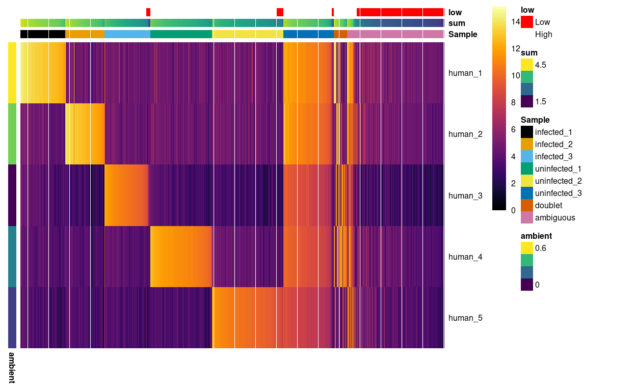
Figure 6: Heatmap of HTO log2(counts + 1) for the droplets. Columns are ordered by sample and then HTO library size. Each droplet (column) is annotated by assigned sample of origin (Sample), the (log10) HTO library size (sum), and whether that is smaller than the a cutoff estimated from the empty droplets. Each HTO (row) is annotated by the (log10) average count of the HTO in the empty droplets (ambient).
Figure 7 is a UMAP plot of the HTO data coloured by the inferred sample.
Show code
set.seed(194)
sce <- runUMAP(sce, altexp = "Antibody Capture", name = "UMAP_HTO")
plotReducedDim(
  sce,
  dimred = "UMAP_HTO",
  colour_by = "Sample",
  point_size = 0.5,
  point_alpha = 1) +
  scale_colour_manual(values = sample_colours, name = "Sample") +
  theme_cowplot() +
  guides(colour = guide_legend(override.aes = list(size = 5)))
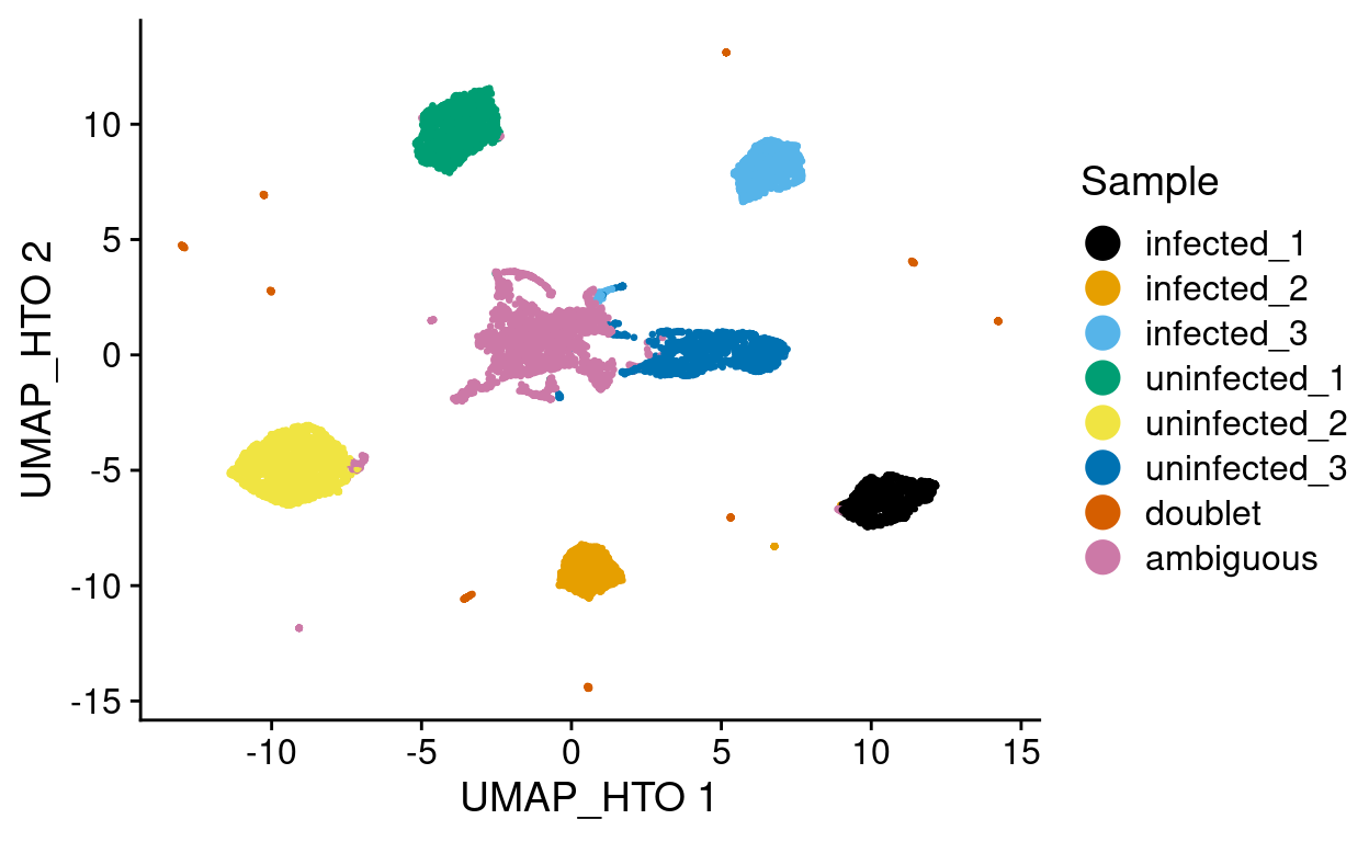
Figure 7: UMAP of HTO data coloured according to the inferred sample.
Summary
James was targeting ~2000 cells / sample. The table below shows that we largely hit that target for the uninfected samples but not so for the infected samples. It also shows that the proportion of droplets that are ambiguous is larger than we would like. These ambiguous droplets include singlets (and doublets) with insufficient HTO sequencing coverage, mis-assigned singlets from the cells labelled with all five HTOs, and samples comprising ambient RNAs and HTOs (aka the ‘soup’ (Young and Behjati, n.d.)).
Show code
knitr::kable(
  as.data.frame(colData(sce)[, c("Sample", "Treatment", "Replicate")]) %>%
    dplyr::count(Sample, Treatment, Replicate),
  caption = "Tabulation of samples by treatment and replicate (mouse). The samples are unpaired.")
| Sample | Treatment | Replicate | n |
|---|---|---|---|
| infected_1 | Infected | 1 | 1479 |
| infected_2 | Infected | 2 | 1283 |
| infected_3 | Infected | 3 | 1509 |
| uninfected_1 | Uninfected | 1 | 2035 |
| uninfected_2 | Uninfected | 2 | 2335 |
| uninfected_3 | Uninfected | 3 | 1664 |
| doublet | NA | NA | 440 |
| ambiguous | NA | NA | 3199 |
Concluding remarks
The processed SingleCellExperiment object is available (see data/SCEs/C057_Cooney.demultiplexed.SCE.rds). This will be used in downstream analyses, e.g., pre-processing.
Additional information
The following are available on request:
- Full CSV tables of any data presented.
- PDF/PNG files of any static plots.
Session info
Show code
sessioninfo::session_info()
─ Session info ─────────────────────────────────────────────────────
 setting  value
 version  R version 4.0.3 (2020-10-10)
 os       CentOS Linux 7 (Core)
 system   x86_64, linux-gnu
 ui       X11
 language (EN)
 collate  en_US.UTF-8
 ctype    en_US.UTF-8
 tz       Australia/Melbourne
 date     2021-03-04

─ Packages ─────────────────────────────────────────────────────────
 ! package              * version  date       lib source
 P assertthat             0.2.1    2019-03-21 [?] CRAN (R 4.0.0)
 P beachmat               2.6.4    2020-12-20 [?] Bioconductor
 P beeswarm               0.2.3    2016-04-25 [?] CRAN (R 4.0.0)
 P Biobase              * 2.50.0   2020-10-27 [?] Bioconductor
   BiocGenerics         * 0.36.0   2020-10-27 [1] Bioconductor
 P BiocManager            1.30.10  2019-11-16 [?] CRAN (R 4.0.0)
 P BiocNeighbors          1.8.2    2020-12-07 [?] Bioconductor
   BiocParallel           1.24.1   2020-11-06 [1] Bioconductor
 P BiocSingular           1.6.0    2020-10-27 [?] Bioconductor
   BiocStyle            * 2.18.1   2020-11-24 [1] Bioconductor
 P bitops                 1.0-6    2013-08-17 [?] CRAN (R 4.0.0)
 P bluster                1.0.0    2020-10-27 [?] Bioconductor
 P bslib                  0.2.4    2021-01-25 [?] CRAN (R 4.0.3)
 P cli                    2.3.1    2021-02-23 [?] CRAN (R 4.0.3)
 P codetools              0.2-18   2020-11-04 [?] CRAN (R 4.0.3)
 P colorspace             2.0-0    2020-11-11 [?] CRAN (R 4.0.3)
 P cowplot              * 1.1.1    2020-12-30 [?] CRAN (R 4.0.3)
 P crayon                 1.4.1    2021-02-08 [?] CRAN (R 4.0.3)
 P DBI                    1.1.1    2021-01-15 [?] CRAN (R 4.0.3)
 P DelayedArray           0.16.2   2021-02-26 [?] Bioconductor
 P DelayedMatrixStats     1.12.3   2021-02-03 [?] Bioconductor
 P digest                 0.6.27   2020-10-24 [?] CRAN (R 4.0.2)
 P distill                1.2      2021-01-13 [?] CRAN (R 4.0.3)
 P downlit                0.2.1    2020-11-04 [?] CRAN (R 4.0.3)
 P dplyr                * 1.0.4    2021-02-02 [?] CRAN (R 4.0.3)
 P dqrng                  0.2.1    2019-05-17 [?] CRAN (R 4.0.0)
 P DropletUtils         * 1.10.3   2021-02-02 [?] Bioconductor
 P edgeR                  3.32.1   2021-01-14 [?] Bioconductor
 P ellipsis               0.3.1    2020-05-15 [?] CRAN (R 4.0.0)
 P evaluate               0.14     2019-05-28 [?] CRAN (R 4.0.0)
 P fansi                  0.4.2    2021-01-15 [?] CRAN (R 4.0.3)
 P farver                 2.1.0    2021-02-28 [?] CRAN (R 4.0.3)
 P generics               0.1.0    2020-10-31 [?] CRAN (R 4.0.3)
 P GenomeInfoDb         * 1.26.2   2020-12-08 [?] Bioconductor
   GenomeInfoDbData       1.2.4    2021-02-04 [1] Bioconductor
 P GenomicRanges        * 1.42.0   2020-10-27 [?] Bioconductor
 P ggbeeswarm             0.6.0    2017-08-07 [?] CRAN (R 4.0.0)
 P ggplot2              * 3.3.3    2020-12-30 [?] CRAN (R 4.0.3)
 P glue                   1.4.2    2020-08-27 [?] CRAN (R 4.0.0)
 P gridExtra              2.3      2017-09-09 [?] CRAN (R 4.0.0)
 P gtable                 0.3.0    2019-03-25 [?] CRAN (R 4.0.0)
 P HDF5Array              1.18.1   2021-02-04 [?] Bioconductor
 P here                 * 1.0.1    2020-12-13 [?] CRAN (R 4.0.3)
 P highr                  0.8      2019-03-20 [?] CRAN (R 4.0.0)
 P htmltools              0.5.1.1  2021-01-22 [?] CRAN (R 4.0.3)
 P igraph                 1.2.6    2020-10-06 [?] CRAN (R 4.0.2)
 P IRanges              * 2.24.1   2020-12-12 [?] Bioconductor
 P irlba                  2.3.3    2019-02-05 [?] CRAN (R 4.0.0)
 P janitor              * 2.1.0    2021-01-05 [?] CRAN (R 4.0.3)
 P jquerylib              0.1.3    2020-12-17 [?] CRAN (R 4.0.3)
 P jsonlite               1.7.2    2020-12-09 [?] CRAN (R 4.0.3)
 P knitr                  1.31     2021-01-27 [?] CRAN (R 4.0.3)
 P labeling               0.4.2    2020-10-20 [?] CRAN (R 4.0.0)
 P lattice                0.20-41  2020-04-02 [?] CRAN (R 4.0.0)
 P lifecycle              1.0.0    2021-02-15 [?] CRAN (R 4.0.3)
   limma                  3.46.0   2020-10-27 [1] Bioconductor
 P locfit                 1.5-9.4  2020-03-25 [?] CRAN (R 4.0.0)
 P lubridate              1.7.10   2021-02-26 [?] CRAN (R 4.0.3)
 P magrittr             * 2.0.1    2020-11-17 [?] CRAN (R 4.0.3)
 P Matrix                 1.3-2    2021-01-06 [?] CRAN (R 4.0.3)
   MatrixGenerics       * 1.2.1    2021-01-30 [1] Bioconductor
 P matrixStats          * 0.58.0   2021-01-29 [?] CRAN (R 4.0.3)
 P munsell                0.5.0    2018-06-12 [?] CRAN (R 4.0.0)
 P pheatmap             * 1.0.12   2019-01-04 [?] CRAN (R 4.0.0)
 P pillar                 1.5.0    2021-02-22 [?] CRAN (R 4.0.3)
 P pkgconfig              2.0.3    2019-09-22 [?] CRAN (R 4.0.0)
 P Polychrome             1.2.6    2020-11-11 [?] CRAN (R 4.0.3)
 P purrr                  0.3.4    2020-04-17 [?] CRAN (R 4.0.0)
 P R.methodsS3            1.8.1    2020-08-26 [?] CRAN (R 4.0.0)
 P R.oo                   1.24.0   2020-08-26 [?] CRAN (R 4.0.0)
 P R.utils                2.10.1   2020-08-26 [?] CRAN (R 4.0.0)
 P R6                     2.5.0    2020-10-28 [?] CRAN (R 4.0.2)
 P RColorBrewer           1.1-2    2014-12-07 [?] CRAN (R 4.0.0)
 P Rcpp                   1.0.6    2021-01-15 [?] CRAN (R 4.0.3)
 P RcppAnnoy              0.0.18   2020-12-15 [?] CRAN (R 4.0.3)
 P RCurl                  1.98-1.2 2020-04-18 [?] CRAN (R 4.0.0)
 P rhdf5                  2.34.0   2020-10-27 [?] Bioconductor
 P rhdf5filters           1.2.0    2020-10-27 [?] Bioconductor
 P Rhdf5lib               1.12.1   2021-01-26 [?] Bioconductor
 P rlang                  0.4.10   2020-12-30 [?] CRAN (R 4.0.3)
 P rmarkdown              2.7      2021-02-19 [?] CRAN (R 4.0.3)
 P rprojroot              2.0.2    2020-11-15 [?] CRAN (R 4.0.3)
 P rsvd                   1.0.3    2020-02-17 [?] CRAN (R 4.0.0)
 P S4Vectors            * 0.28.1   2020-12-09 [?] Bioconductor
 P sass                   0.3.1    2021-01-24 [?] CRAN (R 4.0.3)
 P scales                 1.1.1    2020-05-11 [?] CRAN (R 4.0.0)
 P scater               * 1.18.6   2021-02-26 [?] Bioconductor
 P scatterplot3d          0.3-41   2018-03-14 [?] CRAN (R 4.0.0)
 P scran                * 1.18.5   2021-02-04 [?] Bioconductor
 P scuttle                1.0.4    2020-12-17 [?] Bioconductor
 P sessioninfo            1.1.1    2018-11-05 [?] CRAN (R 4.0.0)
 P SingleCellExperiment * 1.12.0   2020-10-27 [?] Bioconductor
 P snakecase              0.11.0   2019-05-25 [?] CRAN (R 4.0.0)
 P sparseMatrixStats      1.2.1    2021-02-02 [?] Bioconductor
 P statmod                1.4.35   2020-10-19 [?] CRAN (R 4.0.2)
 P stringi                1.5.3    2020-09-09 [?] CRAN (R 4.0.0)
 P stringr                1.4.0    2019-02-10 [?] CRAN (R 4.0.0)
 P SummarizedExperiment * 1.20.0   2020-10-27 [?] Bioconductor
 P tibble                 3.1.0    2021-02-25 [?] CRAN (R 4.0.3)
 P tidyselect             1.1.0    2020-05-11 [?] CRAN (R 4.0.0)
 P utf8                   1.1.4    2018-05-24 [?] CRAN (R 4.0.0)
 P uwot                   0.1.10   2020-12-15 [?] CRAN (R 4.0.3)
 P vctrs                  0.3.6    2020-12-17 [?] CRAN (R 4.0.3)
 P vipor                  0.4.5    2017-03-22 [?] CRAN (R 4.0.0)
 P viridis                0.5.1    2018-03-29 [?] CRAN (R 4.0.0)
 P viridisLite            0.3.0    2018-02-01 [?] CRAN (R 4.0.0)
 P withr                  2.4.1    2021-01-26 [?] CRAN (R 4.0.3)
 P xfun                   0.21     2021-02-10 [?] CRAN (R 4.0.3)
 P XVector                0.30.0   2020-10-27 [?] Bioconductor
 P yaml                   2.2.1    2020-02-01 [?] CRAN (R 4.0.0)
 P zlibbioc               1.36.0   2020-10-27 [?] Bioconductor

[1] /stornext/Projects/score/Analyses/C057_Cooney/renv/library/R-4.0/x86_64-pc-linux-gnu
[2] /tmp/RtmpoUthMU/renv-system-library
[3] /stornext/System/data/apps/R/R-4.0.3/lib64/R/library

 P ── Loaded and on-disk path mismatch.
Lun, A., S. Riesenfeld, T. Andrews, T. P. Dao, T. Gomes, participants in the 1st Human Cell Atlas Jamboree, and J. Marioni. 2018. “Distinguishing Cells from Empty Droplets in Droplet-Based Single-Cell Rna Sequencing Data.” bioRxiv. https://doi.org/10.1101/234872.
Young, MD, and S Behjati. n.d. “SoupX Removes Ambient Rna Contamination from Droplet Based Single Cell Rna Sequencing Data. BioRxiv. 2018.” DOI 10: 303727.
Median-based size factors can adjust for the composition bias that is inherent to the HTO counts; see http://bioconductor.org/books/release/OSCA/integrating-with-protein-abundance.html#cite-seq-median-norm for details.↩︎