Summary
This report excludes samples coming from donors 1-3.
The report begins with some general Setup and is followed by various analyses denoted by a prefix (y):
Setup
Load data
Show code
sce <- readRDS(
  here("data", "SCEs", "C094_Pellicci.mini-bulk.preprocessed.SCE.rds"))
# NOTE: Reorder samples for plots (e.g., heatmaps). Dan requested that the
#       samples be ordered Thymus.S1, Thymus.S2, Thymus.S3, Blood.S3.
sce$tissue <- relevel(sce$tissue, "Thymus")
sce <- sce[, order(sce$tissue, sce$stage, sce$donor)]

# NOTE: Abbreviate stage
levels(sce$stage) <- c("S1", "S2", "S3", "Unknown")
names(sce$colours$stage_colours) <- ifelse(
  grepl("Unknown", names(sce$colours$stage_colours)),
  "Unknown",
  substr(names(sce$colours$stage_colours), 1, 2))

# Convoluted way to add tech rep ID
sce$rep <- dplyr::group_by(
  as.data.frame(colData(sce)),
  tissue, stage, donor) %>%
  dplyr::mutate(rep = dplyr::row_number()) %>%
  dplyr::pull(rep)
colnames(sce) <- interaction(
  sce$sample,
  sce$stage,
  sce$rep,
  drop = TRUE,
  lex.order = TRUE)

# Restrict analysis to read counts
assays(sce) <- list(counts = assay(sce, "read_counts"))
outdir <- here("output", "DEGs", "excluding_donors_1-3")
dir.create(outdir, recursive = TRUE)
Gene filtering
We filter the genes to only retain protein coding genes.
Sample filtering
We exclude all samples from donors 1-3.
Show code
sce <- sce[, !sce$donor %in% 1:3]

colData(sce) <- droplevels(colData(sce))
Show code
# Some useful colours
plate_number_colours <- setNames(
  unique(sce$colours$plate_number_colours),
  unique(names(sce$colours$plate_number_colours)))[levels(sce$plate_number)]
sample_type_colours <- setNames(
  unique(sce$colours$sample_type_colours),
  unique(names(sce$colours$sample_type_colours)))[levels(sce$sample_type)]
sample_gate_colours <- setNames(
  unique(sce$colours$sample_gate_colours),
  unique(names(sce$colours$sample_gate_colours)))[levels(sce$sample_gate)]
stage_colours <- setNames(
  unique(sce$colours$stage_colours),
  unique(names(sce$colours$stage_colours)))[levels(sce$stage)]
sequencing_run_colours <- setNames(
  unique(sce$colours$sequencing_run_colours),
  unique(names(sce$colours$sequencing_run_colours)))[levels(sce$sequencing_run)]
tissue_colours <- setNames(
  unique(sce$colours$tissue_colours),
  unique(names(sce$colours$tissue_colours)))[levels(sce$tissue)]
donor_colours <- setNames(
  unique(sce$colours$donor_colours),
  unique(names(sce$colours$donor_colours)))[levels(sce$donor)]
sample_colours <- setNames(
  unique(sce$colours$sample_colours),
  unique(names(sce$colours$sample_colours)))[levels(sce$sample)]
Create DGEList objects
Show code
x <- DGEList(
  counts = as.matrix(counts(sce)),
  samples = colData(sce),
  group = interaction(sce$tissue, sce$stage, drop = TRUE, lex.order = TRUE),
  genes = flattenDF(rowData(sce)))
# Remove genes with zero counts.
x <- x[rowSums(x$counts) > 0, ]
Show code
y <- sumTechReps(
  x,
  interaction(sce$sample, sce$stage, drop = TRUE, lex.order = TRUE))
Gene filtering
For each analysis, shown are the number of genes that have sufficient counts to test for DE (TRUE) or not (FALSE).
y
Show code
y_keep_exprs <- filterByExpr(y, group = y$samples$group, min.count = 5)
# NOTE: Keep a copy of the unfiltered data for violin plots.
y_ <- y
y <- y[y_keep_exprs, , keep.lib.sizes = FALSE]
table(y_keep_exprs)
y_keep_exprs
FALSE  TRUE
 3441 11054
Normalization
Normalization with upper-quartile (UQ) normalization.
Show code
# NOTE: Prefer to use upper-quartile (on basis of analysis in C086_Kinkel) but
#       this cannot be applied to `x` for this dataset.
x <- calcNormFactors(x, method = "TMM")
y <- calcNormFactors(y, method = "upperquartile")
Aggregation of technical replicates
We have 2 - 6 technical replicates from each biological replicate. Ideally, the technical replicates are very similar to one another when view on an MDS plot. However, Figure 1 shows that:
- Samples roughly cluster somewhat by
stageandtissue - Some of the technical replicates are more variable than we would like
- Those ‘outlier’ samples have smaller library sizes
Show code
x_mds <- plotMDS(x, plot = FALSE)
x_df <- cbind(data.frame(x = x_mds$x, y = x_mds$y), x$samples)
rownames(x_df) <- colnames(x)

p1 <- ggplot(
  aes(x = x, y = y, colour = tissue, label = rownames(x_df)),
  data = x_df) +
  geom_point() +
  theme_cowplot(font_size = 6) +
  xlab("Leading logFC dim 1") +
  ylab("Leading logFC dim 2") +
  scale_colour_manual(values = tissue_colours)
p2 <- ggplot(
  aes(x = x, y = y, colour = donor, label = rownames(x_df)),
  data = x_df) +
  geom_point() +
  theme_cowplot(font_size = 6) +
  xlab("Leading logFC dim 1") +
  ylab("Leading logFC dim 2") +
  scale_colour_manual(values = donor_colours) +
  guides(col = guide_legend(ncol = 2))
p3 <- ggplot(
  aes(x = x, y = y, colour = plate_number, label = rownames(x_df)),
  data = x_df) +
  geom_point() +
  theme_cowplot(font_size = 6) +
  xlab("Leading logFC dim 1") +
  ylab("Leading logFC dim 2") +
  scale_colour_manual(values = plate_number_colours)
p4 <- ggplot(
  aes(x = x, y = y, colour = sample, label = rownames(x_df)),
  data = x_df) +
  geom_point() +
  theme_cowplot(font_size = 6) +
  xlab("Leading logFC dim 1") +
  ylab("Leading logFC dim 2") +
  scale_colour_manual(values = sample_colours) +
  guides(col = guide_legend(ncol = 2))
p5 <- ggplot(
  aes(x = x, y = y, colour = sample_type, label = rownames(x_df)),
  data = x_df) +
  geom_point() +
  theme_cowplot(font_size = 6) +
  xlab("Leading logFC dim 1") +
  ylab("Leading logFC dim 2") +
  scale_colour_manual(values = sample_type_colours)
p6 <- ggplot(
  aes(x = x, y = y, colour = sequencing_run, label = rownames(x_df)),
  data = x_df) +
  geom_point() +
  theme_cowplot(font_size = 6) +
  xlab("Leading logFC dim 1") +
  ylab("Leading logFC dim 2") +
  scale_colour_manual(values = sequencing_run_colours)
p7 <- ggplot(
  aes(x = x, y = y, colour = stage, label = rownames(x_df)),
  data = x_df) +
  geom_point() +
  theme_cowplot(font_size = 6) +
  xlab("Leading logFC dim 1") +
  ylab("Leading logFC dim 2") +
  scale_colour_manual(values = stage_colours)
p8 <- ggplot(
  aes(x = x, y = y, colour = sample_gate, label = rownames(x_df)),
  data = x_df) +
  geom_point() +
  theme_cowplot(font_size = 6) +
  xlab("Leading logFC dim 1") +
  ylab("Leading logFC dim 2") +
  scale_colour_manual(values = sample_gate_colours)
p9 <- ggplot(
  aes(x = x, y = y, colour = log10(lib.size), label = rownames(x_df)),
  data = x_df) +
  geom_point() +
  theme_cowplot(font_size = 6) +
  scale_colour_viridis_c() +
  xlab("Leading logFC dim 1") +
  ylab("Leading logFC dim 2")

p1 + p2 + p3 + p4 + p5 + p6 + p7 + p8 + p9 + plot_layout(ncol = 3)
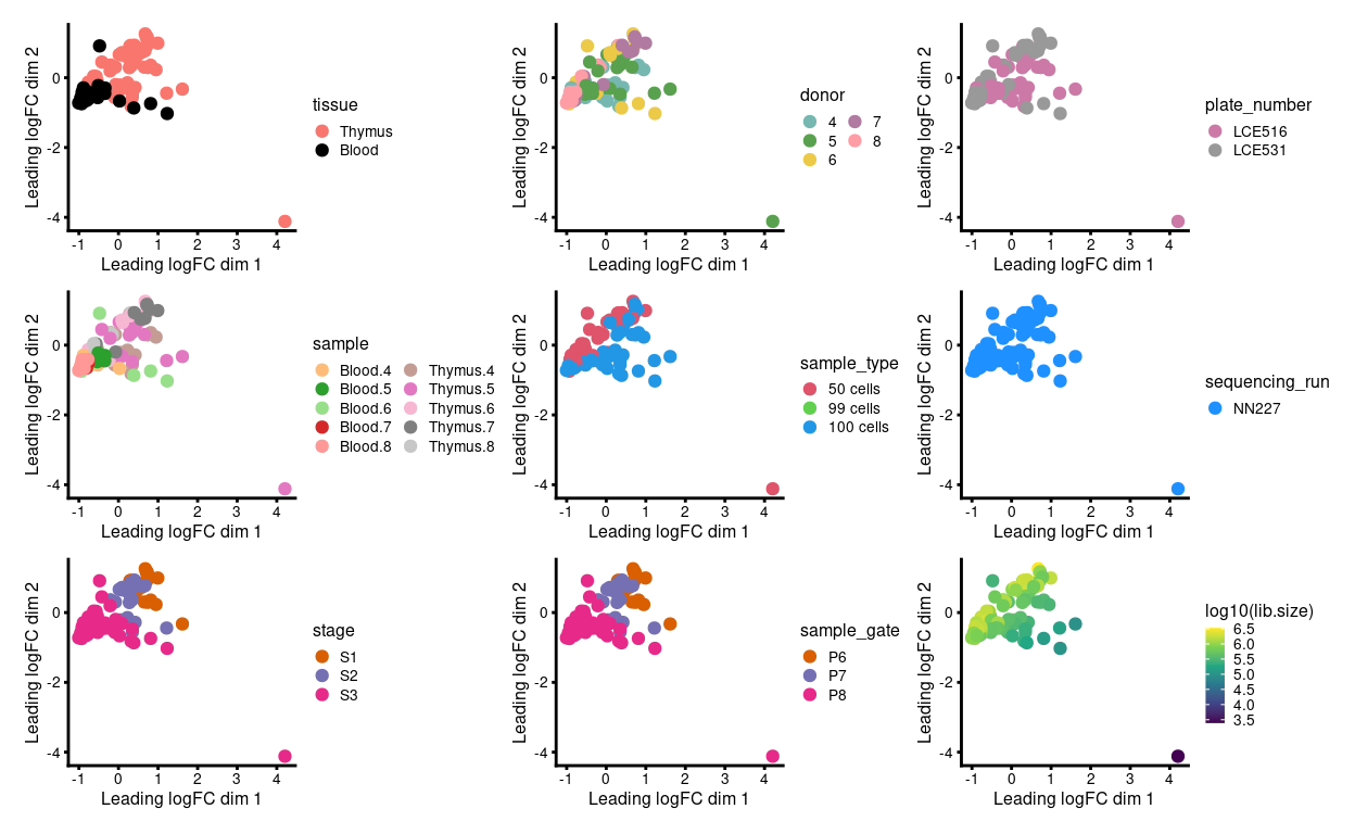
Figure 1: MDS plots of individual technical replicates coloured by various experimental factors.
Although we could analyse the data at the level of technical replicates, this is more complicated. It will make our life easier by aggregating these technical replicates so that we have 1 sample per biological replicate. To aggregate technical replicates we simply sum their counts.
Figure 2 shows the MDS plot after aggregating the technical replicates. We observe that:
- Much of the variation is associated with library size
- There is no strong
donor/plate_numberbatch effect
Show code
y_mds <- plotMDS(y, plot = FALSE)
y_df <- cbind(data.frame(x = y_mds$x, y = y_mds$y), y$samples)
rownames(y_df) <- colnames(y)

p1 <- ggplot(
  aes(x = x, y = y, colour = tissue, label = rownames(y_df)),
  data = y_df) +
  geom_point() +
  theme_cowplot(font_size = 6) +
  xlab("Leading logFC dim 1") +
  ylab("Leading logFC dim 2") +
  scale_colour_manual(values = tissue_colours)
p2 <- ggplot(
  aes(x = x, y = y, colour = donor, label = rownames(y_df)),
  data = y_df) +
  geom_point() +
  theme_cowplot(font_size = 6) +
  xlab("Leading logFC dim 1") +
  ylab("Leading logFC dim 2") +
  scale_colour_manual(values = donor_colours) +
  guides(col = guide_legend(ncol = 2))
p3 <- ggplot(
  aes(x = x, y = y, colour = plate_number, label = rownames(y_df)),
  data = y_df) +
  geom_point() +
  theme_cowplot(font_size = 6) +
  xlab("Leading logFC dim 1") +
  ylab("Leading logFC dim 2") +
  scale_colour_manual(values = plate_number_colours)
p4 <- ggplot(
  aes(x = x, y = y, colour = sample, label = rownames(y_df)),
  data = y_df) +
  geom_point() +
  theme_cowplot(font_size = 6) +
  xlab("Leading logFC dim 1") +
  ylab("Leading logFC dim 2") +
  scale_colour_manual(values = sample_colours) +
  guides(col = guide_legend(ncol = 2))
# NOTE: Not showing sample_type because we ignored it when aggregating the
#       tech reps.
# p5 <- ggplot(
#   aes(x = x, y = y, colour = sample_type, label = rownames(y_df)),
#   data = y_df) +
#   geom_point() +
#   geom_text_repel(size = 2) +
#   theme_cowplot(font_size = 6) +
#   xlab("Leading logFC dim 1") +
#   ylab("Leading logFC dim 2") +
#   scale_colour_manual(values = sample_type_colours)
p6 <- ggplot(
  aes(x = x, y = y, colour = sequencing_run, label = rownames(y_df)),
  data = y_df) +
  geom_point() +
  theme_cowplot(font_size = 6) +
  xlab("Leading logFC dim 1") +
  ylab("Leading logFC dim 2") +
  scale_colour_manual(values = sequencing_run_colours)
p7 <- ggplot(
  aes(x = x, y = y, colour = stage, label = rownames(y_df)),
  data = y_df) +
  geom_point() +
  theme_cowplot(font_size = 6) +
  xlab("Leading logFC dim 1") +
  ylab("Leading logFC dim 2") +
  scale_colour_manual(values = stage_colours)
p8 <- ggplot(
  aes(x = x, y = y, colour = sample_gate, label = rownames(y_df)),
  data = y_df) +
  geom_point() +
  theme_cowplot(font_size = 6) +
  xlab("Leading logFC dim 1") +
  ylab("Leading logFC dim 2") +
  scale_colour_manual(values = sample_gate_colours)
p9 <- ggplot(
  aes(x = x, y = y, colour = log10(lib.size), label = rownames(y_df)),
  data = y_df) +
  geom_point() +
  theme_cowplot(font_size = 6) +
  scale_colour_viridis_c() +
  xlab("Leading logFC dim 1") +
  ylab("Leading logFC dim 2")

p1 + p2 + p3 + p4 + p6 + p7 + p8 + p9 + plot_layout(ncol = 3)
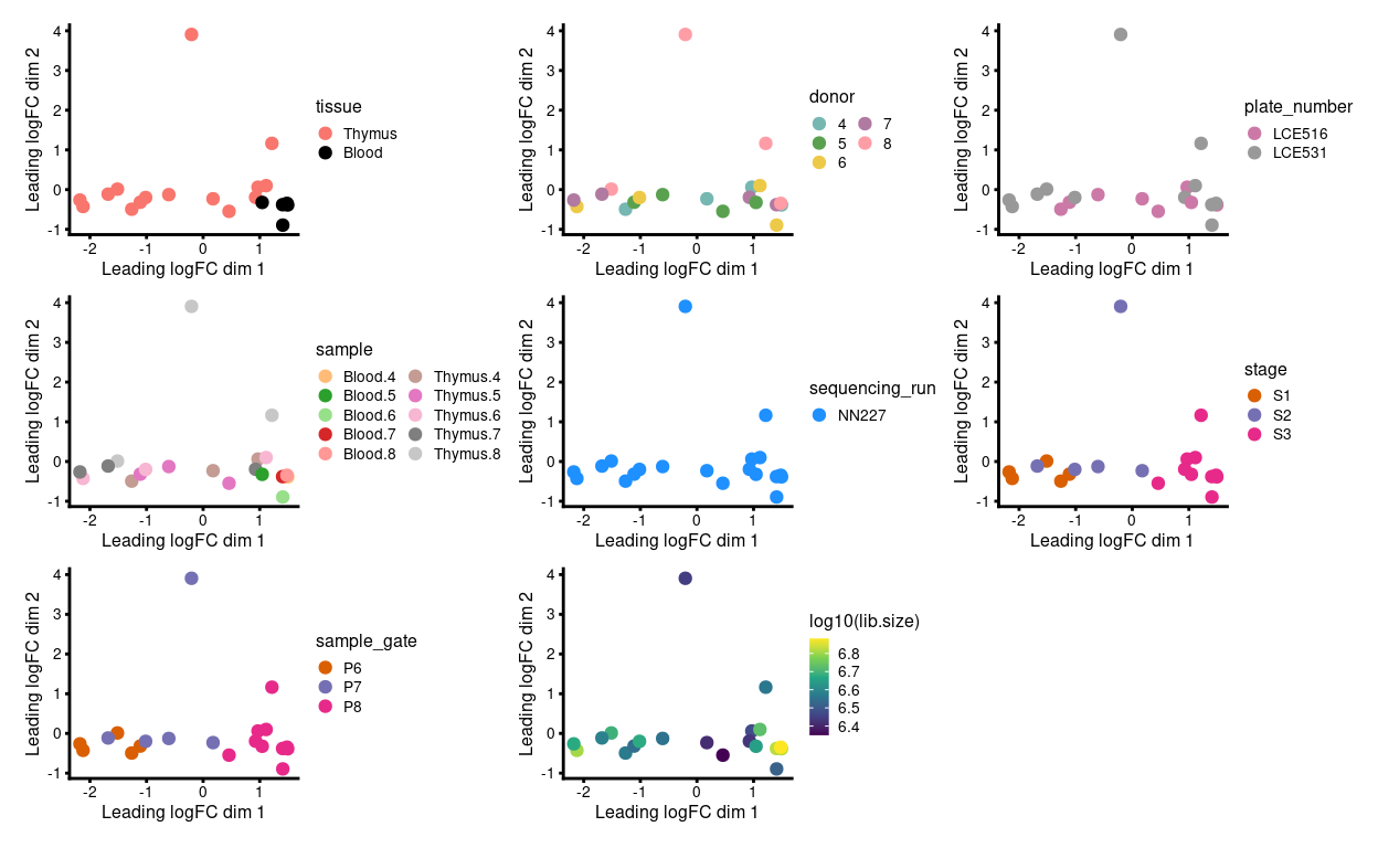
Figure 2: MDS plots of aggregated technical replicates coloured by various experimental factors.
Fortunately, the plates were designed such that the comparisons of interest can be made within each, which protects us to an extent from plate-to-plate variation. Figure 3 is an MDS plot after removing the batch effect due to donor1. We can more clearly observe the stage- and tissue-specific variation.
Show code
y_mds <- plotMDS(
  removeBatchEffect(
    cpm(y, log = TRUE),
    batch = y$samples$donor,
    design = model.matrix(~group, y$samples)),
  plot = FALSE)
y_df <- cbind(data.frame(x = y_mds$x, y = y_mds$y), y$samples)
rownames(y_df) <- colnames(y)

p1 <- ggplot(
  aes(x = x, y = y, colour = tissue, label = rownames(y_df)),
  data = y_df) +
  geom_point() +
  theme_cowplot(font_size = 6) +
  xlab("Leading logFC dim 1") +
  ylab("Leading logFC dim 2") +
  scale_colour_manual(values = tissue_colours)
p2 <- ggplot(
  aes(x = x, y = y, colour = donor, label = rownames(y_df)),
  data = y_df) +
  geom_point() +
  theme_cowplot(font_size = 6) +
  xlab("Leading logFC dim 1") +
  ylab("Leading logFC dim 2") +
  scale_colour_manual(values = donor_colours) +
  guides(col = guide_legend(ncol = 2))
p3 <- ggplot(
  aes(x = x, y = y, colour = plate_number, label = rownames(y_df)),
  data = y_df) +
  geom_point() +
  theme_cowplot(font_size = 6) +
  xlab("Leading logFC dim 1") +
  ylab("Leading logFC dim 2") +
  scale_colour_manual(values = plate_number_colours)
p4 <- ggplot(
  aes(x = x, y = y, colour = sample, label = rownames(y_df)),
  data = y_df) +
  geom_point() +
  theme_cowplot(font_size = 6) +
  xlab("Leading logFC dim 1") +
  ylab("Leading logFC dim 2") +
  scale_colour_manual(values = sample_colours) +
  guides(col = guide_legend(ncol = 2))
# NOTE: Not showing sample_type because we ignored it when aggregating the
#       tech reps.
# p5 <- ggplot(
#   aes(x = x, y = y, colour = sample_type, label = rownames(y_df)),
#   data = y_df) +
#   geom_point() +
#   geom_text_repel(size = 2) +
#   theme_cowplot(font_size = 6) +
#   xlab("Leading logFC dim 1") +
#   ylab("Leading logFC dim 2") +
#   scale_colour_manual(values = sample_type_colours)
p6 <- ggplot(
  aes(x = x, y = y, colour = sequencing_run, label = rownames(y_df)),
  data = y_df) +
  geom_point() +
  theme_cowplot(font_size = 6) +
  xlab("Leading logFC dim 1") +
  ylab("Leading logFC dim 2") +
  scale_colour_manual(values = sequencing_run_colours)
p7 <- ggplot(
  aes(x = x, y = y, colour = stage, label = rownames(y_df)),
  data = y_df) +
  geom_point() +
  theme_cowplot(font_size = 6) +
  xlab("Leading logFC dim 1") +
  ylab("Leading logFC dim 2") +
  scale_colour_manual(values = stage_colours)
p8 <- ggplot(
  aes(x = x, y = y, colour = sample_gate, label = rownames(y_df)),
  data = y_df) +
  geom_point() +
  theme_cowplot(font_size = 6) +
  xlab("Leading logFC dim 1") +
  ylab("Leading logFC dim 2") +
  scale_colour_manual(values = sample_gate_colours)
p9 <- ggplot(
  aes(x = x, y = y, colour = log10(lib.size), label = rownames(y_df)),
  data = y_df) +
  geom_point() +
  theme_cowplot(font_size = 6) +
  scale_colour_viridis_c() +
  xlab("Leading logFC dim 1") +
  ylab("Leading logFC dim 2")

p1 + p2 + p3 + p4 + p6 + p7 + p8 + p9 + plot_layout(ncol = 3)
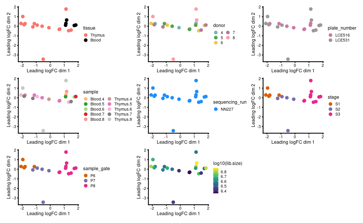
Figure 3: MDS plots of aggregated technical replicates coloured by various experimental factors.
Analysis of aggregated technical replicates
Violin plots
Show code
y_ <- calcNormFactors(y_, method = "upperquartile")
se <- SingleCellExperiment(
  assays = list(
    logCPM = cpm(y_, log = TRUE),
    `batch-corrected logCPM` = removeBatchEffect(
    cpm(y_, log = TRUE),
    batch = y_$samples$donor,
    design = model.matrix(~group, y_$samples))),
  colData = y_$samples,
  rowData = y_$genes)

genes <- c(
  # TFs
  "BCL11B", "LEF1", "TBET" = "TBX21", "EOMES",
  # Chemokines
  "CCR5", "CCR9", "CXCR3", "CXCR6", "CCR6",
  # Surface molecules
  "CD28", "CD44", "CD26" = "DPP4", "CD94" = "KLRD1", "IL18RAP",
  # Markers used for gating.
  "CD4", "CD161" = "KLRB1")

# NOTE: Dan requested particular group colours (email 2021-09-07). I manually
#       matched these colours to the examples in figure Dan sent.
group_colours <- c(
  "Thymus.S1" = "#3954a1",
  "Thymus.S2" = "#94c643",
  "Thymus.S3" = "#ec2327",
  "Blood.S3" = "#6a539f")
Dan requested violin plots of specific genes (email 2021-08-12), listed below. I’ve added in CD4 and KLRB1 (CD161) for good measure.
Show code
dir.create(file.path(outdir, "violin_plots"))

genes_df <- data.frame(
  `Gene name supplied by Dan` = ifelse(names(genes) == "", genes, names(genes)),
  `Gene name in dataset` = unname(genes),
  Detected = genes %in% rownames(y_),
  Tested = genes %in% rownames(y),
  check.names = FALSE)
knitr::kable(
  genes_df,
  caption = "Genes requested by Dan for violin plots, their corresponding name in the dataset, whether they are detected in the mini-bulk data (`Detected`), and whether they are sufficiently expressed to be tested in the DE analysis (`Tested`).")
| Gene name supplied by Dan | Gene name in dataset | Detected | Tested |
|---|---|---|---|
| BCL11B | BCL11B | TRUE | TRUE |
| LEF1 | LEF1 | TRUE | TRUE |
| TBET | TBX21 | TRUE | TRUE |
| EOMES | EOMES | TRUE | TRUE |
| CCR5 | CCR5 | TRUE | TRUE |
| CCR9 | CCR9 | TRUE | TRUE |
| CXCR3 | CXCR3 | TRUE | TRUE |
| CXCR6 | CXCR6 | TRUE | TRUE |
| CCR6 | CCR6 | TRUE | FALSE |
| CD28 | CD28 | TRUE | TRUE |
| CD44 | CD44 | TRUE | TRUE |
| CD26 | DPP4 | TRUE | TRUE |
| CD94 | KLRD1 | TRUE | TRUE |
| IL18RAP | IL18RAP | TRUE | TRUE |
| CD4 | CD4 | TRUE | TRUE |
| CD161 | KLRB1 | TRUE | TRUE |
Figures 4 and 5 show the expression of the Detected genes, either as \(log(CPM)\) or as batch-corrected \(log(CPM)\).
Show code
# NOTE: The following is a workaround to the lack of support for tabsets in
#       distill (see https://github.com/rstudio/distill/issues/11 and
#       https://github.com/rstudio/distill/issues/11#issuecomment-692142414 in
#       particular).
xaringanExtra::use_panelset()
logCPM
Show code
scater::plotExpression(
  se,
  features = intersect(genes_df$`Gene name in dataset`, rownames(se)),
  x = "group",
  exprs_values = "logCPM",
  scales = "free_y",
  ncol = 4,
  colour_by = "group",
  point_alpha = 1) +
  theme(axis.title.x = element_blank(), axis.text.x = element_blank()) +
  scale_colour_manual(values = group_colours, name = "group")
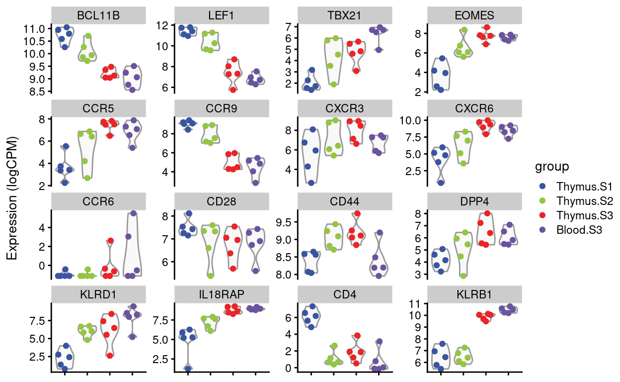
Figure 4: Expression of Dan’s requested genes.
Show code
pdf(file.path(outdir, "violin_plots", "logCPM.pdf"), height = 5, width = 6)
for (i in seq_len(nrow(genes_df))) {
  g <- intersect(genes_df$`Gene name in dataset`[i], rownames(se))
  if (length(g)) {
    p <- scater::plotExpression(
      se,
      features = g,
      x = "group",
      exprs_values = "logCPM",
      colour_by = "group",
      point_alpha = 1,
      point_size = 3,
      show_violin = FALSE,
      show_median = TRUE) +
      scale_colour_manual(values = group_colours, name = "group")
    print(p)
  }
}
dev.off()
Batch-corrected logCPM
Show code
scater::plotExpression(
  se,
  features = intersect(genes_df$`Gene name in dataset`, rownames(se)),
  x = "group",
  exprs_values = "batch-corrected logCPM",
  scales = "free_y",
  ncol = 4,
  colour_by = "group",
  point_alpha = 1) +
  theme(axis.title.x = element_blank(), axis.text.x = element_blank()) +
  scale_colour_manual(values = group_colours, name = "group")
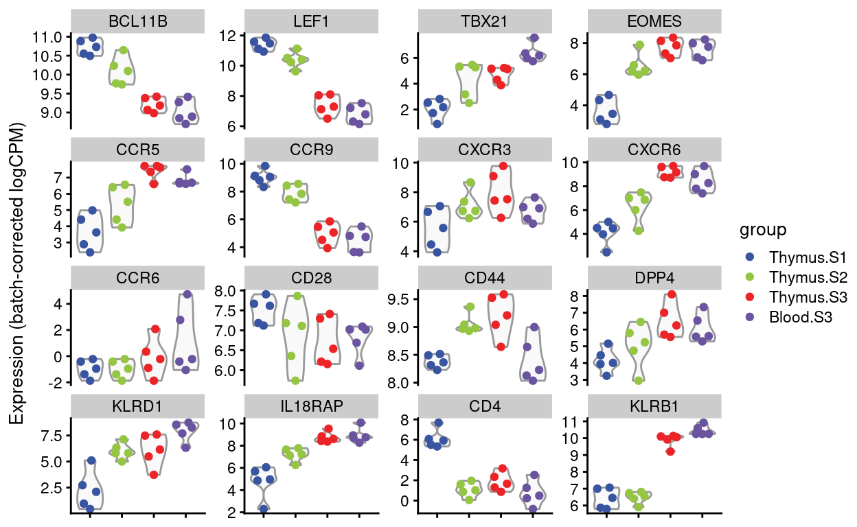
Figure 5: Expression of Dan’s requested genes.
Show code
pdf(
  file.path(outdir, "violin_plots", "batch-corrected_logCPM.pdf"),
  height = 5,
  width = 6)
for (i in seq_len(nrow(genes_df))) {
  g <- intersect(genes_df$`Gene name in dataset`[i], rownames(se))
  if (length(g)) {
    p <- scater::plotExpression(
      se,
      features = g,
      x = "group",
      exprs_values = "batch-corrected logCPM",
      scales = "free_y",
      ncol = 4,
      colour_by = "group",
      point_alpha = 1,
      point_size = 3,
      show_violin = FALSE,
      show_median = TRUE) +
      scale_colour_manual(values = group_colours, name = "group")
    print(p)
  }
}
dev.off()
DE analysis
Fit a model using edgeR with a term for group and donor.
Show code
y <- estimateDisp(y, y_design)
par(mfrow = c(1, 1))
plotBCV(y)
Show code
y_dgeglm <- glmFit(y, y_design)
y_contrast <- makeContrasts(
  Thymus.S3_vs_Thymus.S1 = Thymus.S3 - Thymus.S1,
  Thymus.S2_vs_Thymus.S1 = Thymus.S2 - Thymus.S1,
  Thymus.S3_vs_Thymus.S2 = Thymus.S3 - Thymus.S2,
  Thymus.S3_vs_Blood.S3 = Thymus.S3 - Blood.S3,
  levels = y_design)

y_dt <- lapply(colnames(y_contrast), function(j) {
  dgelrt <- glmLRT(y_dgeglm, contrast = y_contrast[, j])
  decideTests(dgelrt)
})
names(y_dt) <- colnames(y_contrast)
do.call(cbind, lapply(y_dt, summary)) %>%
    knitr::kable(caption = "Number of DEGs (FDR < 0.05)")
| -1Thymus.S1 1Thymus.S3 | -1Thymus.S1 1Thymus.S2 | -1Thymus.S2 1Thymus.S3 | 1Thymus.S3 -1Blood.S3 | |
|---|---|---|---|---|
| Down | 309 | 19 | 81 | 30 |
| NotSig | 10476 | 10989 | 10929 | 11004 |
| Up | 269 | 46 | 44 | 20 |
MD plots
Figure 6 - 9 are MD plots in each comparison.
Show code
# NOTE: The following is a workaround to the lack of support for tabsets in
#       distill (see https://github.com/rstudio/distill/issues/11 and
#       https://github.com/rstudio/distill/issues/11#issuecomment-692142414 in
#       particular).
xaringanExtra::use_panelset()
Thymus.S3_vs_Thymus.S1
Show code
j <- "Thymus.S3_vs_Thymus.S1"
dgelrt <- glmLRT(y_dgeglm, contrast = y_contrast[, j])

par(mfrow = c(1, 2))
plotMD(dgelrt, legend = "bottomright")
abline(h = 0, lty = 2, col = "dodgerBlue")
plotMD(
  dgelrt,
  status = ifelse(
    rownames(dgelrt) == "CD4",
    "CD4",
    ifelse(rownames(dgelrt) == "KLRB1", "KLRB1", "other")),
  hl.col = c("orange", "dodgerBlue"),
  legend = "bottomright",
  hl.cex = 2)
abline(h = 0, lty = 2, col = "dodgerBlue")
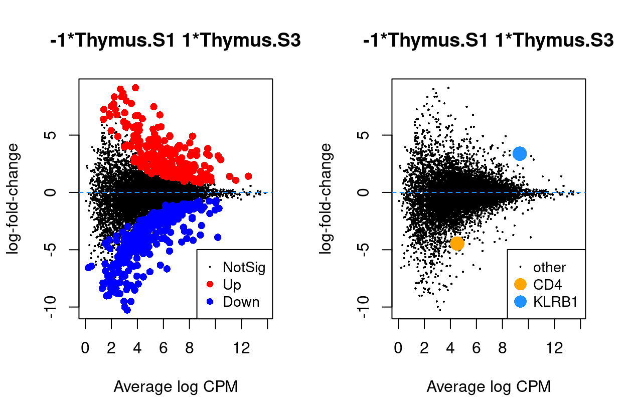
Figure 6: MD plots highlighting DEGs and stage marker genes CD4 and KLRB1 (CD161)
Thymus.S2_vs_Thymus.S1
Show code
j <- "Thymus.S2_vs_Thymus.S1"
dgelrt <- glmLRT(y_dgeglm, contrast = y_contrast[, j])

par(mfrow = c(1, 2))
plotMD(dgelrt, legend = "bottomright")
abline(h = 0, lty = 2, col = "dodgerBlue")
plotMD(
  dgelrt,
  status = ifelse(
    rownames(dgelrt) == "CD4",
    "CD4",
    ifelse(rownames(dgelrt) == "KLRB1", "KLRB1", "other")),
  hl.col = c("orange", "dodgerBlue"),
  legend = "bottomright",
  hl.cex = 2)
abline(h = 0, lty = 2, col = "dodgerBlue")
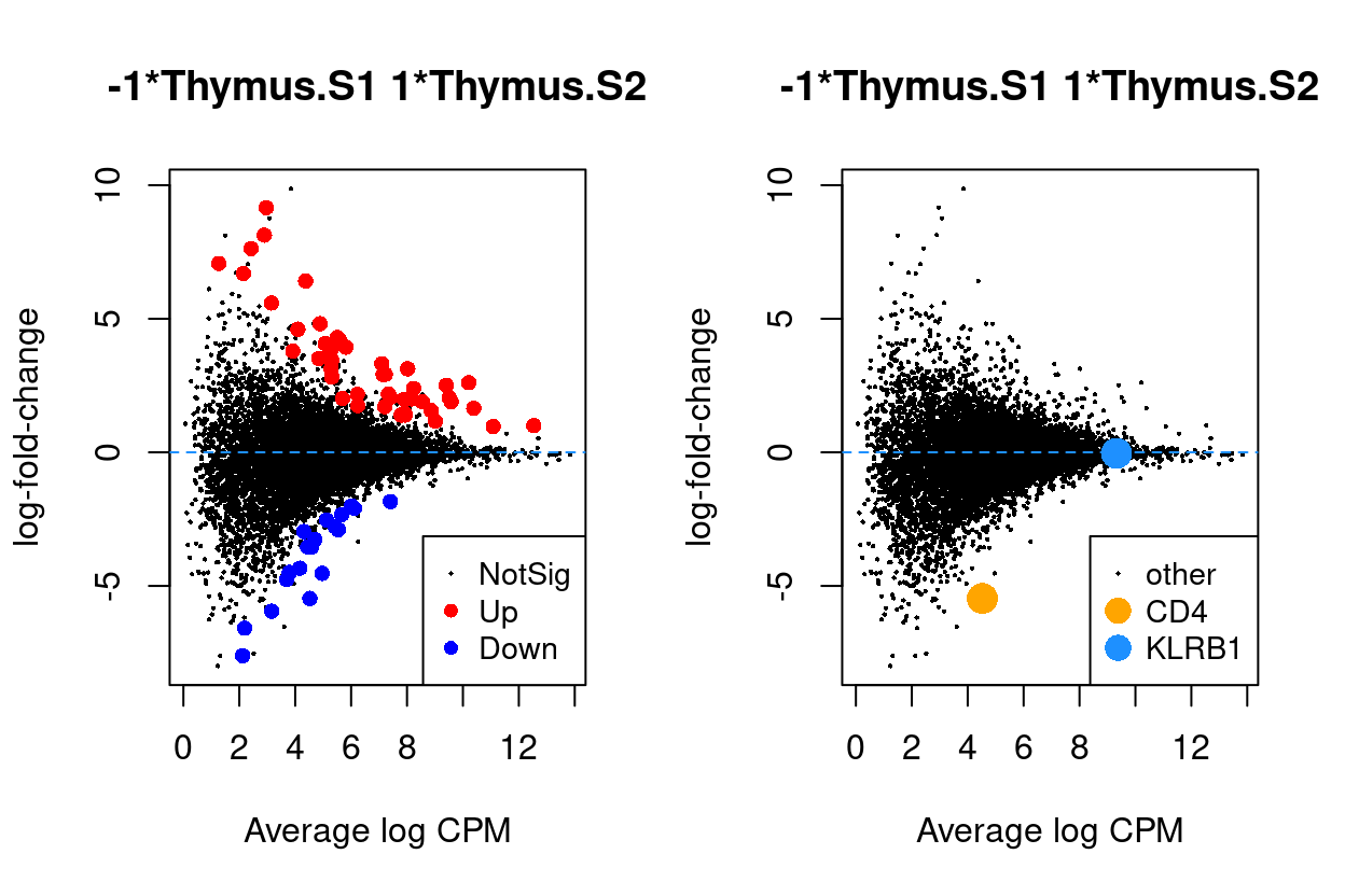
Figure 7: MD plots highlighting DEGs and stage marker genes CD4 and KLRB1 (CD161)
Thymus.S3_vs_Thymus.S2
Show code
j <- "Thymus.S3_vs_Thymus.S2"
dgelrt <- glmLRT(y_dgeglm, contrast = y_contrast[, j])

par(mfrow = c(1, 2))
plotMD(dgelrt, legend = "bottomright")
abline(h = 0, lty = 2, col = "dodgerBlue")
plotMD(
  dgelrt,
  status = ifelse(
    rownames(dgelrt) == "CD4",
    "CD4",
    ifelse(rownames(dgelrt) == "KLRB1", "KLRB1", "other")),
  hl.col = c("orange", "dodgerBlue"),
  legend = "bottomright",
  hl.cex = 2)
abline(h = 0, lty = 2, col = "dodgerBlue")
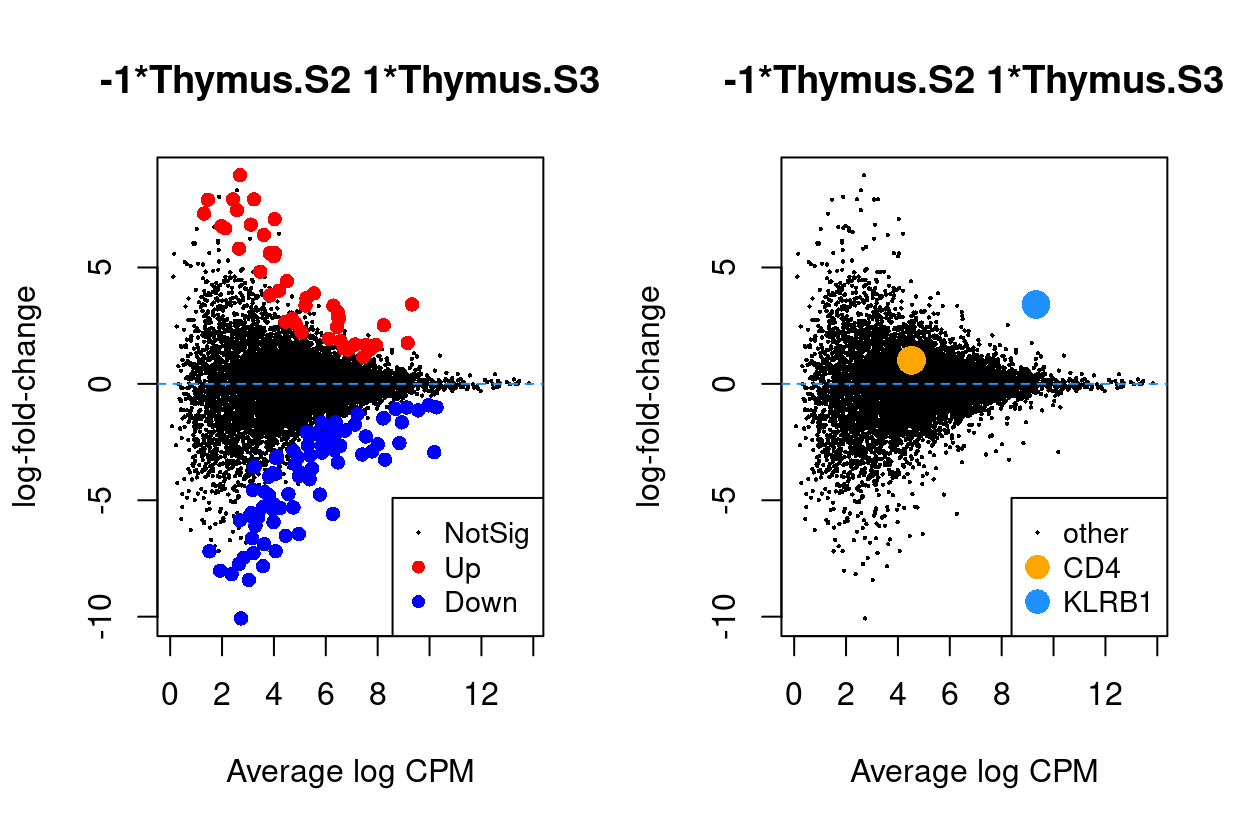
Figure 8: MD plots highlighting DEGs and stage marker genes CD4 and KLRB1 (CD161)
Thymus.S3_vs_Blood.S3
Show code
j <- "Thymus.S3_vs_Blood.S3"
dgelrt <- glmLRT(y_dgeglm, contrast = y_contrast[, j])

par(mfrow = c(1, 2))
plotMD(dgelrt, legend = "bottomright")
abline(h = 0, lty = 2, col = "dodgerBlue")
plotMD(
  dgelrt,
  status = ifelse(
    rownames(dgelrt) == "CD4",
    "CD4",
    ifelse(rownames(dgelrt) == "KLRB1", "KLRB1", "other")),
  hl.col = c("orange", "dodgerBlue"),
  legend = "bottomright",
  hl.cex = 2)
abline(h = 0, lty = 2, col = "dodgerBlue")
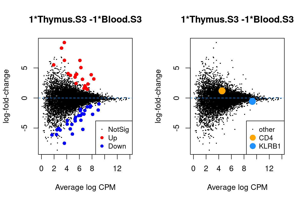
Figure 9: MD plots highlighting DEGs and stage marker genes CD4 and KLRB1 (CD161)
Interactive Glimma MD plots of the differential expression results are available from output/DEGs/excluding_donors_1-3/glimma-plots/.
Show code
lapply(colnames(y_contrast), function(j) {
  dgelrt <- glmLRT(y_dgeglm, contrast = y_contrast[, j])
  glMDPlot(
    x = dgelrt,
    counts = y,
    anno = y$genes,
    display.columns = c("ENSEMBL.SYMBOL"),
    groups = y$samples$group,
    samples = colnames(y),
    status = y_dt[[j]],
    transform = TRUE,
    sample.cols = y$samples$colours.stage_colours,
    path = outdir,
    html = paste0(j, ".aggregated_tech_reps.md-plot"),
    main = j,
    launch = FALSE)
})
Tables
The following tables give the DEGs in each comparison.
Show code
# NOTE: The following is a workaround to the lack of support for tabsets in
#       distill (see https://github.com/rstudio/distill/issues/11 and
#       https://github.com/rstudio/distill/issues/11#issuecomment-692142414 in
#       particular).
xaringanExtra::use_panelset()
Thymus.S3_vs_Thymus.S1
Show code
j <- "Thymus.S3_vs_Thymus.S1"
dgelrt <- glmLRT(y_dgeglm, contrast = y_contrast[, j])
tt <- topTags(dgelrt, p.value = 0.05, n = Inf)
if (nrow(tt)) {
  tt$table[, c("logFC", "logCPM", "LR", "PValue", "FDR")] %>%
    DT::datatable(caption = "DEGs (FDR < 0.05)") %>%
    DT::formatSignif(
      c("logFC", "logCPM", "LR", "PValue", "FDR"),
      digits = 3)
}
Thymus.S2_vs_Thymus.S1
Show code
j <- "Thymus.S2_vs_Thymus.S1"
dgelrt <- glmLRT(y_dgeglm, contrast = y_contrast[, j])
tt <- topTags(dgelrt, p.value = 0.05, n = Inf)
if (nrow(tt)) {
  tt$table[, c("logFC", "logCPM", "LR", "PValue", "FDR")] %>%
    DT::datatable(caption = "DEGs (FDR < 0.05)") %>%
    DT::formatSignif(
      c("logFC", "logCPM", "LR", "PValue", "FDR"),
      digits = 3)
}
Thymus.S3_vs_Thymus.S2
Show code
j <- "Thymus.S3_vs_Thymus.S2"
dgelrt <- glmLRT(y_dgeglm, contrast = y_contrast[, j])
tt <- topTags(dgelrt, p.value = 0.05, n = Inf)
if (nrow(tt)) {
  tt$table[, c("logFC", "logCPM", "LR", "PValue", "FDR")] %>%
    DT::datatable(caption = "DEGs (FDR < 0.05)") %>%
    DT::formatSignif(
      c("logFC", "logCPM", "LR", "PValue", "FDR"),
      digits = 3)
}
Thymus.S3_vs_Blood.S3
Show code
j <- "Thymus.S3_vs_Blood.S3"
dgelrt <- glmLRT(y_dgeglm, contrast = y_contrast[, j])
tt <- topTags(dgelrt, p.value = 0.05, n = Inf)
if (nrow(tt)) {
  tt$table[, c("logFC", "logCPM", "LR", "PValue", "FDR")] %>%
    DT::datatable(caption = "DEGs (FDR < 0.05)") %>%
    DT::formatSignif(
      c("logFC", "logCPM", "LR", "PValue", "FDR"),
      digits = 3)
}
CSV file of results available from output/DEGs/excluding_donors_1-3/aggregated_tech_reps.DEGs.csv.gz.
Show code
lapply(colnames(y_contrast), function(j) {
  dgelrt <- glmLRT(y_dgeglm, contrast = y_contrast[, j])
  gzout <- gzfile(
    description = file.path(
      outdir,
      paste0(j, ".aggregated_tech_reps.DEGs.csv.gz")),
    open = "wb")
  write.csv(
    topTags(dgelrt, n = Inf),
  gzout,
  # NOTE: quote = TRUE needed because some fields contain commas.
  quote = TRUE,
  row.names = FALSE)
  close(gzout)
})
Heatmaps
Figure 10 - 13 are heatmaps showing the expression of the DEGs in each comparison.
Show code
# NOTE: The following is a workaround to the lack of support for tabsets in
#       distill (see https://github.com/rstudio/distill/issues/11 and
#       https://github.com/rstudio/distill/issues/11#issuecomment-692142414 in
#       particular).
xaringanExtra::use_panelset()
Thymus.S3_vs_Thymus.S1
Show code
j <- "Thymus.S3_vs_Thymus.S1"
dgelrt <- glmLRT(y_dgeglm, contrast = y_contrast[, j])
tt <- topTags(dgelrt, p.value = 0.05, n = Inf)
pheatmap(
  removeBatchEffect(
    cpm(y, log = TRUE),
    batch = y$samples$donor,
    design = model.matrix(~group, y$samples))[head(rownames(tt), 50), ],
  cluster_rows = TRUE,
  cluster_cols = FALSE,
  color = hcl.colors(101, "Blue-Red 3"),
  breaks = seq(-3, 3, length.out = 101),
  scale = "row",
  annotation_col = data.frame(
    tissue = y$samples$tissue,
    stage = y$samples$stage,
    row.names = colnames(y)),
  annotation_colors = list(
    tissue = tissue_colours,
    stage = stage_colours),
  main = j,
  fontsize = 6)
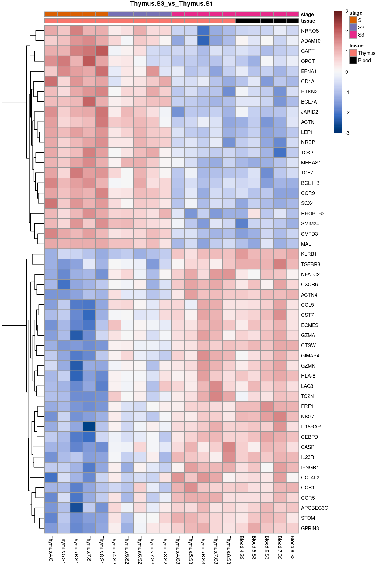
Figure 10: Heatmap of batch-corrected logCPM values for the top-50 DEGs.
Thymus.S2_vs_Thymus.S1
Show code
j <- "Thymus.S2_vs_Thymus.S1"
dgelrt <- glmLRT(y_dgeglm, contrast = y_contrast[, j])
tt <- topTags(dgelrt, p.value = 0.05, n = Inf)
pheatmap(
  removeBatchEffect(
    cpm(y, log = TRUE),
    batch = y$samples$donor,
    design = model.matrix(~group, y$samples))[head(rownames(tt), 50), ],
  cluster_rows = TRUE,
  cluster_cols = FALSE,
  color = hcl.colors(101, "Blue-Red 3"),
  breaks = seq(-3, 3, length.out = 101),
  scale = "row",
  annotation_col = data.frame(
    tissue = y$samples$tissue,
    stage = y$samples$stage,
    row.names = colnames(y)),
  annotation_colors = list(
    tissue = tissue_colours,
    stage = stage_colours),
  main = j,
  fontsize = 6)
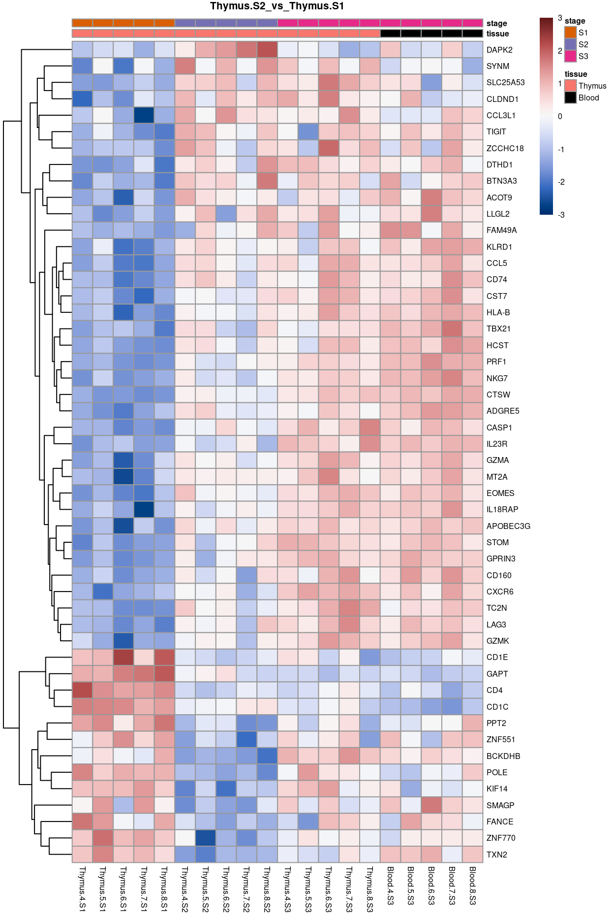
Figure 11: Heatmap of batch-corrected logCPM values for the top-50 DEGs.
Thymus.S3_vs_Thymus.S2
Show code
j <- "Thymus.S3_vs_Thymus.S2"
dgelrt <- glmLRT(y_dgeglm, contrast = y_contrast[, j])
tt <- topTags(dgelrt, p.value = 0.05, n = Inf)
pheatmap(
  removeBatchEffect(
    cpm(y, log = TRUE),
    batch = y$samples$donor,
    design = model.matrix(~group, y$samples))[head(rownames(tt), 50), ],
  cluster_rows = TRUE,
  cluster_cols = FALSE,
  color = hcl.colors(101, "Blue-Red 3"),
  breaks = seq(-3, 3, length.out = 101),
  scale = "row",
  annotation_col = data.frame(
    tissue = y$samples$tissue,
    stage = y$samples$stage,
    row.names = colnames(y)),
  annotation_colors = list(
    tissue = tissue_colours,
    stage = stage_colours),
  main = j,
  fontsize = 6)
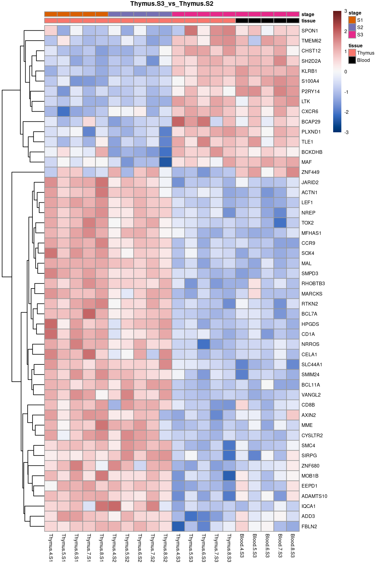
Figure 12: Heatmap of batch-corrected logCPM values for the top-50 DEGs.
Thymus.S3_vs_Blood.S3
Show code
j <- "Thymus.S3_vs_Blood.S3"
dgelrt <- glmLRT(y_dgeglm, contrast = y_contrast[, j])
tt <- topTags(dgelrt, p.value = 0.05, n = Inf)
pheatmap(
  removeBatchEffect(
    cpm(y, log = TRUE),
    batch = y$samples$donor,
    design = model.matrix(~group, y$samples))[head(rownames(tt), 50), ],
  cluster_rows = TRUE,
  cluster_cols = FALSE,
  color = hcl.colors(101, "Blue-Red 3"),
  breaks = seq(-3, 3, length.out = 101),
  scale = "row",
  annotation_col = data.frame(
    tissue = y$samples$tissue,
    stage = y$samples$stage,
    row.names = colnames(y)),
  annotation_colors = list(
    tissue = tissue_colours,
    stage = stage_colours),
  main = j,
  fontsize = 6)
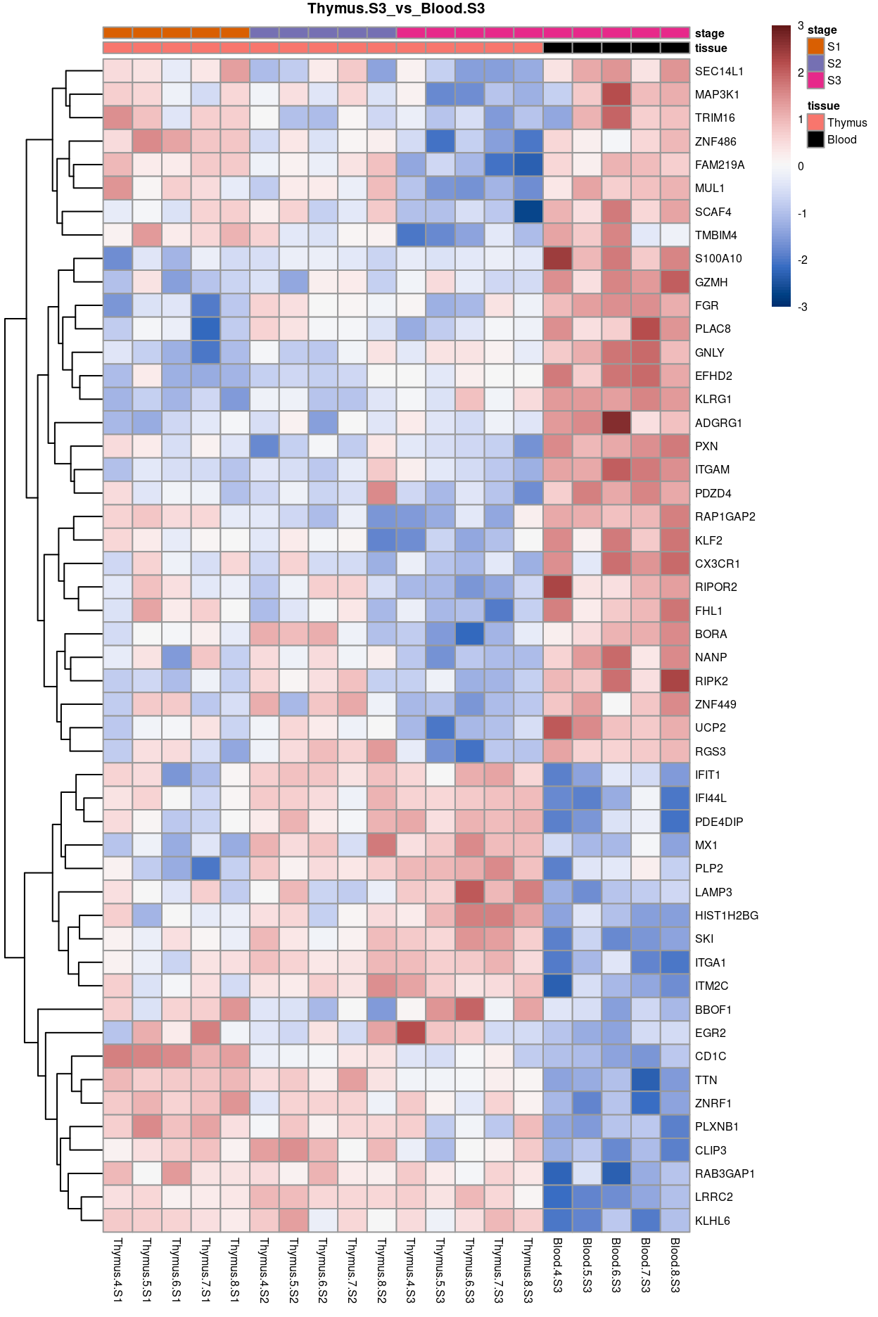
Figure 13: Heatmap of batch-corrected logCPM values for the top-50 DEGs.
Gene set tests
Gene set testing is commonly used to interpret the differential expression results in a biological context. Here we apply various gene set tests to the DEG lists.
goana
We use the goana() function from the limma R/Bioconductor package to test for over-representation of gene ontology (GO) terms in each DEG list.
Show code
list_of_go <- lapply(colnames(y_contrast), function(j) {
  dgelrt <- glmLRT(y_dgeglm, contrast = y_contrast[, j])

  go <- goana(
    de = dgelrt,
    geneid = sapply(strsplit(dgelrt$genes$NCBI.ENTREZID, "; "), "[[", 1),
    species = "Hs")
  gzout <- gzfile(
    description = file.path(
      outdir,
      paste0(j, ".aggregated_tech_reps.goana.csv.gz")),
    open = "wb")
  write.csv(
    topGO(go, number = Inf),
    gzout,
    row.names = TRUE)
  close(gzout)
  go
})
names(list_of_go) <- colnames(y_contrast)
CSV files of the results are available from output/DEGs/excluding_donors_1-3/.
An example of the results are shown below.
Show code
topGO(list_of_go[[1]]) %>%
  knitr::kable(
    caption = '`goana()` produces a table with a row for each GO term and the following columns: **Term** (GO term); **Ont** (ontology that the GO term belongs to. Possible values are "BP", "CC" and "MF"); **N** (number of genes in the GO term); **Up** (number of up-regulated differentially expressed genes); **Down** (number of down-regulated differentially expressed genes); **P.Up** (p-value for over-representation of GO term in up-regulated genes); **P.Down** (p-value for over-representation of GO term in down-regulated genes)')
| Term | Ont | N | Up | Down | P.Up | P.Down | |
|---|---|---|---|---|---|---|---|
| GO:0006955 | immune response | BP | 1244 | 101 | 57 | 0.0e+00 | 0.0001050 |
| GO:0002376 | immune system process | BP | 1873 | 120 | 84 | 0.0e+00 | 0.0000032 |
| GO:0006952 | defense response | BP | 890 | 74 | 37 | 0.0e+00 | 0.0094939 |
| GO:0009605 | response to external stimulus | BP | 1479 | 93 | 57 | 0.0e+00 | 0.0066895 |
| GO:0045087 | innate immune response | BP | 516 | 51 | 20 | 0.0e+00 | 0.0872265 |
| GO:0005886 | plasma membrane | CC | 2389 | 121 | 99 | 0.0e+00 | 0.0000104 |
| GO:0071944 | cell periphery | CC | 2454 | 122 | 101 | 0.0e+00 | 0.0000109 |
| GO:0009986 | cell surface | CC | 345 | 41 | 25 | 0.0e+00 | 0.0000127 |
| GO:0007166 | cell surface receptor signaling pathway | BP | 1666 | 96 | 72 | 0.0e+00 | 0.0000717 |
| GO:0004888 | transmembrane signaling receptor activity | MF | 261 | 35 | 15 | 0.0e+00 | 0.0066305 |
| GO:0098542 | defense response to other organism | BP | 628 | 54 | 24 | 0.0e+00 | 0.0740711 |
| GO:0043207 | response to external biotic stimulus | BP | 812 | 62 | 29 | 0.0e+00 | 0.1028408 |
| GO:0051707 | response to other organism | BP | 812 | 62 | 29 | 0.0e+00 | 0.1028408 |
| GO:0048731 | system development | BP | 2546 | 91 | 135 | 3.4e-05 | 0.0000000 |
| GO:0060089 | molecular transducer activity | MF | 356 | 40 | 23 | 0.0e+00 | 0.0001639 |
| GO:0038023 | signaling receptor activity | MF | 356 | 40 | 23 | 0.0e+00 | 0.0001639 |
| GO:0050896 | response to stimulus | BP | 4947 | 186 | 178 | 0.0e+00 | 0.0000029 |
| GO:0009607 | response to biotic stimulus | BP | 834 | 62 | 29 | 0.0e+00 | 0.1302868 |
| GO:0007165 | signal transduction | BP | 3178 | 139 | 122 | 0.0e+00 | 0.0000257 |
| GO:0031224 | intrinsic component of membrane | CC | 2362 | 115 | 80 | 0.0e+00 | 0.0311423 |
kegga
We use the kegga() function from the limma R/Bioconductor package to test for over-representation of KEGG pathways in each DEG list.
Show code
list_of_kegg <- lapply(colnames(y_contrast), function(j) {
  dgelrt <- glmLRT(y_dgeglm, contrast = y_contrast[, j])

  kegg <- kegga(
    de = dgelrt,
    geneid = sapply(strsplit(dgelrt$genes$NCBI.ENTREZID, "; "), "[[", 1),
    species = "Hs")
  gzout <- gzfile(
    description = file.path(
      outdir,
      paste0(j, ".aggregated_tech_reps.kegga.csv.gz")),
    open = "wb")
  write.csv(
    topKEGG(kegg, number = Inf),
    gzout,
    row.names = TRUE)
  close(gzout)
  kegg
})
names(list_of_kegg) <- colnames(y_contrast)
CSV files of the results are available from output/DEGs/excluding_donors_1-3/.
An example of the results are shown below.
Show code
topKEGG(list_of_kegg[[1]]) %>%
  knitr::kable(
    caption = '`kegga()` produces a table with a row for each KEGG pathway ID and the following columns: **Pathway** (KEGG pathway); **N** (number of genes in the GO term); **Up** (number of up-regulated differentially expressed genes); **Down** (number of down-regulated differentially expressed genes); **P.Up** (p-value for over-representation of KEGG pathway in up-regulated genes); **P.Down** (p-value for over-representation of KEGG pathway in down-regulated genes)')
| Pathway | N | Up | Down | P.Up | P.Down | |
|---|---|---|---|---|---|---|
| path:hsa04060 | Cytokine-cytokine receptor interaction | 88 | 20 | 6 | 0.0000000 | 0.0370027 |
| path:hsa04061 | Viral protein interaction with cytokine and cytokine receptor | 38 | 12 | 2 | 0.0000000 | 0.2888525 |
| path:hsa04650 | Natural killer cell mediated cytotoxicity | 87 | 16 | 1 | 0.0000000 | 0.9167013 |
| path:hsa04640 | Hematopoietic cell lineage | 49 | 3 | 13 | 0.1172099 | 0.0000000 |
| path:hsa05332 | Graft-versus-host disease | 26 | 9 | 1 | 0.0000000 | 0.5231950 |
| path:hsa05320 | Autoimmune thyroid disease | 24 | 7 | 1 | 0.0000012 | 0.4952095 |
| path:hsa05330 | Allograft rejection | 25 | 7 | 1 | 0.0000016 | 0.5094011 |
| path:hsa04940 | Type I diabetes mellitus | 27 | 7 | 1 | 0.0000028 | 0.5366023 |
| path:hsa05167 | Kaposi sarcoma-associated herpesvirus infection | 144 | 14 | 2 | 0.0000111 | 0.9157103 |
| path:hsa04062 | Chemokine signaling pathway | 120 | 12 | 1 | 0.0000356 | 0.9677193 |
| path:hsa05163 | Human cytomegalovirus infection | 162 | 14 | 2 | 0.0000419 | 0.9447182 |
| path:hsa05321 | Inflammatory bowel disease | 40 | 7 | 4 | 0.0000448 | 0.0251161 |
| path:hsa04612 | Antigen processing and presentation | 56 | 8 | 3 | 0.0000586 | 0.2072610 |
| path:hsa04514 | Cell adhesion molecules | 72 | 9 | 9 | 0.0000599 | 0.0001725 |
| path:hsa05165 | Human papillomavirus infection | 205 | 15 | 7 | 0.0001504 | 0.3527293 |
| path:hsa05170 | Human immunodeficiency virus 1 infection | 165 | 12 | 3 | 0.0007224 | 0.8463277 |
| path:hsa04659 | Th17 cell differentiation | 88 | 7 | 9 | 0.0056519 | 0.0007827 |
| path:hsa05164 | Influenza A | 122 | 10 | 2 | 0.0007955 | 0.8609872 |
| path:hsa05169 | Epstein-Barr virus infection | 167 | 12 | 4 | 0.0008037 | 0.6937346 |
| path:hsa05146 | Amoebiasis | 42 | 2 | 6 | 0.2737915 | 0.0010394 |
camera with MSigDB gene sets
We use the camera() function from the limma R/Bioconductor package to test whether a set of genes is highly ranked relative to other genes in terms of differential expression, accounting for inter-gene correlation. Specifically, we test using gene sets from MSigDB, namely:
- H: hallmark gene sets are coherently expressed signatures derived by aggregating many MSigDB gene sets to represent well-defined biological states or processes.
- C2: curated gene sets from online pathway databases, publications in PubMed, and knowledge of domain experts.
- C7: immunologic signature gene sets represent cell states and perturbations within the immune system.
Show code
# NOTE: Using BiocFileCache to avoid re-downloading these gene sets everytime
#       the report is rendered.
library(BiocFileCache)
bfc <- BiocFileCache()
# NOTE: Creating list of gene sets in this slightly convoluted way so that each
#       gene set name is prepended by its origin (e.g. H, C2, or C7).
msigdb <- do.call(
  c,
  list(
    H = readRDS(
      bfcrpath(
        bfc,
        "http://bioinf.wehi.edu.au/MSigDB/v7.1/Hs.h.all.v7.1.entrez.rds")),
    C2 = readRDS(
      bfcrpath(
        bfc,
        "http://bioinf.wehi.edu.au/MSigDB/v7.1/Hs.c2.all.v7.1.entrez.rds")),
    C7 = readRDS(
      bfcrpath(
        bfc,
        "http://bioinf.wehi.edu.au/MSigDB/v7.1/Hs.c7.all.v7.1.entrez.rds"))))

y_idx <- ids2indices(
  msigdb,
  id = sapply(strsplit(y$genes$NCBI.ENTREZID, "; "), "[[", 1))
list_of_camera <- lapply(colnames(y_contrast), function(j) {
  cam <- camera(
    y = y,
    index = y_idx,
    design = y_design,
    contrast = y_contrast[, j])
  gzout <- gzfile(
    description = file.path(
      outdir,
      paste0(j, ".aggregated_tech_reps.camera.csv.gz")),
    open = "wb")
  write.csv(
    cam,
    gzout,
    row.names = TRUE)
  close(gzout)
  cam
})
CSV files of the results are available from output/DEGs/excluding_donors_1-3/.
An example of the results are shown below.
Show code
head(list_of_camera[[1]]) %>%
  knitr::kable(
    caption = '`camera()` produces a table with a row for each gene set (prepended by which MSigDB collection it comes from) and the following columns: **NGenes** (number of genes in set); **Direction** (direction of change); **PValue** (two-tailed p-value); **FDR** (Benjamini and Hochberg FDR adjusted p-value).')
| NGenes | Direction | PValue | FDR | |
|---|---|---|---|---|
| C7.GSE26495_NAIVE_VS_PD1HIGH_CD8_TCELL_DN | 188 | Up | 0 | 0 |
| C7.GSE26495_NAIVE_VS_PD1LOW_CD8_TCELL_DN | 191 | Up | 0 | 0 |
| C2.HAHTOLA_SEZARY_SYNDROM_DN | 36 | Up | 0 | 0 |
| C7.GSE45739_UNSTIM_VS_ACD3_ACD28_STIM_WT_CD4_TCELL_DN | 191 | Up | 0 | 0 |
| C7.GSE5542_UNTREATED_VS_IFNA_TREATED_EPITHELIAL_CELLS_6H_UP | 154 | Up | 0 | 0 |
| C7.GSE45739_UNSTIM_VS_ACD3_ACD28_STIM_NRAS_KO_CD4_TCELL_DN | 154 | Up | 0 | 0 |
Dan’s gene lists
Dan requested testing if the ‘SLAM-SAP-FYN pathway’ was differentially expressed in each comparison. Genes in this pathway are listed below.
Show code
dan_df <- data.frame(
  `Gene name supplied by Dan` = unname(
    ifelse(
      unlist(lapply(dan, names)) == "",
      unlist(dan),
      unlist(lapply(dan, names)))),
  `Gene name in dataset` = unname(unlist(dan)),
  Detected = unlist(dan) %in% rownames(y_),
  Tested = unlist(dan) %in% rownames(y),
  check.names = FALSE)
knitr::kable(
  dan_df,
  caption = "Genes in 'SLAM-SAP-FYN' pathway requested by Dan for gene set analysis, their corresponding name in the dataset, whether they are detected in the mini-bulk data (`Detected`), and whether they are sufficiently expressed to be tested in the DE analysis (`Tested`).")
| Gene name supplied by Dan | Gene name in dataset | Detected | Tested |
|---|---|---|---|
| SLAMF1 | SLAMF1 | TRUE | TRUE |
| SLAMF2 | CD48 | TRUE | TRUE |
| SLAMF3 | LY9 | TRUE | TRUE |
| SLAMF4 | CD244 | TRUE | TRUE |
| SLAMF5 | CD84 | TRUE | TRUE |
| SLAMF6 | SLAMF6 | TRUE | TRUE |
| SLAMF7 | SLAMF7 | TRUE | TRUE |
| SLAMF8 | SLAMF8 | TRUE | TRUE |
| SLAMF9 | SLAMF9 | FALSE | FALSE |
| FYN | FYN | TRUE | TRUE |
| SAP | SH2D1A | TRUE | TRUE |
We use the fry() function from the edgeR R/Bioconductor package to perform a self-contained gene set test against the null hypothesis that none of the genes in the set are differentially expressed.
Show code
# NOTE: The following is a workaround to the lack of support for tabsets in
#       distill (see https://github.com/rstudio/distill/issues/11 and
#       https://github.com/rstudio/distill/issues/11#issuecomment-692142414 in
#       particular).
xaringanExtra::use_panelset()
Thymus.S3_vs_Thymus.S1
Show code
j <- "Thymus.S3_vs_Thymus.S1"
fry(
  y,
  index = y_index,
  design = y_design,
  contrast = y_contrast[, j]) %>%
  knitr::kable(
    caption = "Results of applying `fry()` to the RNA-seq differential expression results using the supplied gene sets. A significant 'Up' P-value means that the differential expression results found in the RNA-seq data are positively correlated with the expression signature from the corresponding gene set. Conversely, a significant 'Down' P-value means that the differential expression log-fold-changes are negatively correlated with the expression signature from the corresponding gene set. A significant 'Mixed' P-value means that the genes in the set tend to be differentially expressed without regard for direction.")
| NGenes | Direction | PValue | PValue.Mixed | |
|---|---|---|---|---|
| SLAM-SAP-FYN pathway | 10 | Up | 0.0249367 | 1.77e-05 |
Thymus.S2_vs_Thymus.S1
Show code
j <- "Thymus.S2_vs_Thymus.S1"
fry(
  y,
  index = y_index,
  design = y_design,
  contrast = y_contrast[, j]) %>%
  knitr::kable(
    caption = "Results of applying `fry()` to the RNA-seq differential expression results using the supplied gene sets. A significant 'Up' P-value means that the differential expression results found in the RNA-seq data are positively correlated with the expression signature from the corresponding gene set. Conversely, a significant 'Down' P-value means that the differential expression log-fold-changes are negatively correlated with the expression signature from the corresponding gene set. A significant 'Mixed' P-value means that the genes in the set tend to be differentially expressed without regard for direction.")
| NGenes | Direction | PValue | PValue.Mixed | |
|---|---|---|---|---|
| SLAM-SAP-FYN pathway | 10 | Up | 0.1087838 | 0.3310179 |
Thymus.S3_vs_Thymus.S2
Show code
j <- "Thymus.S3_vs_Thymus.S2"
fry(
  y,
  index = y_index,
  design = y_design,
  contrast = y_contrast[, j]) %>%
  knitr::kable(
    caption = "Results of applying `fry()` to the RNA-seq differential expression results using the supplied gene sets. A significant 'Up' P-value means that the differential expression results found in the RNA-seq data are positively correlated with the expression signature from the corresponding gene set. Conversely, a significant 'Down' P-value means that the differential expression log-fold-changes are negatively correlated with the expression signature from the corresponding gene set. A significant 'Mixed' P-value means that the genes in the set tend to be differentially expressed without regard for direction.")
| NGenes | Direction | PValue | PValue.Mixed | |
|---|---|---|---|---|
| SLAM-SAP-FYN pathway | 10 | Up | 0.3293575 | 0.0037329 |
Thymus.S3_vs_Blood.S3
Show code
j <- "Thymus.S3_vs_Blood.S3"
fry(
  y,
  index = y_index,
  design = y_design,
  contrast = y_contrast[, j]) %>%
  knitr::kable(
    caption = "Results of applying `fry()` to the RNA-seq differential expression results using the supplied gene sets. A significant 'Up' P-value means that the differential expression results found in the RNA-seq data are positively correlated with the expression signature from the corresponding gene set. Conversely, a significant 'Down' P-value means that the differential expression log-fold-changes are negatively correlated with the expression signature from the corresponding gene set. A significant 'Mixed' P-value means that the genes in the set tend to be differentially expressed without regard for direction.")
| NGenes | Direction | PValue | PValue.Mixed | |
|---|---|---|---|---|
| SLAM-SAP-FYN pathway | 10 | Up | 0.8627486 | 0.8238979 |
Visualisation
Show code
j <- "Thymus.S3_vs_Thymus.S1"
dgelrt <- glmLRT(y_dgeglm, contrast = y_contrast[, j])

term <- "C2.REACTOME_INTERFERON_ALPHA_BETA_SIGNALING"
library(org.Hs.eg.db)
key <- msigdb[[term]]
tmp <- AnnotationDbi::select(
  org.Hs.eg.db,
  key = key,
  columns = "SYMBOL",
  keytype = "ENTREZID")
y_index <- ids2indices(unique(tmp$SYMBOL), rownames(y))
We can visualise the expression of the genes in any given set and in any given comparison using a ‘barcode plot’ and/or by highlighting those genes on the MD plot. Such figures are often included in publications.
Figure 14 gives an example showing the expression of genes in the C2.REACTOME_INTERFERON_ALPHA_BETA_SIGNALING MSigDB gene set in the Thymus.S3_vs_Thymus.S1 comparison.
Show code
par(mfrow = c(1, 2))
y_status <- rep("Other", nrow(dgelrt))
y_status[y_index[[1]]] <- "In"
plotMD(
  dgelrt,
  status = y_status,
  values = "In",
  hl.col = "red",
  legend = "bottomright",
  main = term,
  cex.main = 0.6)
abline(h = 0, col = "darkgrey")
barcodeplot(statistics = dgelrt$table$logFC, index = y_index[[1]])
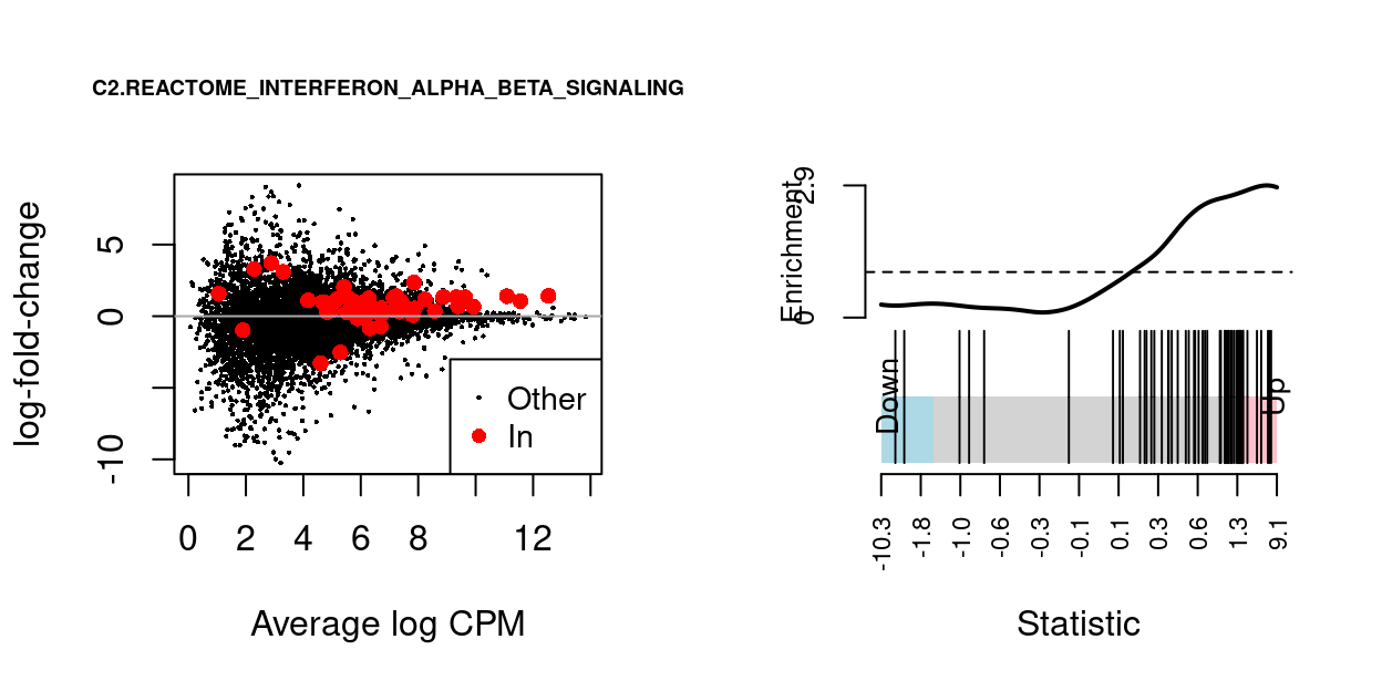
Figure 14: MD-plot and barcode plot of genes in MSigDB set C2.REACTOME_INTERFERON_ALPHA_BETA_SIGNALING. For the barcode plot, genes are represented by bars and are ranked from left to right by increasing log-fold change. This forms the barcode-like pattern. The line (or worm) above the barcode shows the relative local enrichment of the vertical bars in each part of the plot. The dotted horizontal line indicates neutral enrichment; the worm above the dotted line shows enrichment while the worm below the dotted line shows depletion.
Session info
Show code
sessioninfo::session_info()
─ Session info ─────────────────────────────────────────────────────
 setting  value
 version  R version 4.0.3 (2020-10-10)
 os       CentOS Linux 7 (Core)
 system   x86_64, linux-gnu
 ui       X11
 language (EN)
 collate  en_US.UTF-8
 ctype    en_US.UTF-8
 tz       Australia/Melbourne
 date     2021-10-06

─ Packages ─────────────────────────────────────────────────────────
 ! package              * version  date       lib
 P annotate               1.68.0   2020-10-27 [?]
 P AnnotationDbi        * 1.52.0   2020-10-27 [?]
 P assertthat             0.2.1    2019-03-21 [?]
 P beachmat               2.6.4    2020-12-20 [?]
 P beeswarm               0.3.1    2021-03-07 [?]
 P Biobase              * 2.50.0   2020-10-27 [?]
 P BiocFileCache        * 1.14.0   2020-10-27 [?]
 P BiocGenerics         * 0.36.0   2020-10-27 [?]
 P BiocManager            1.30.12  2021-03-28 [?]
 P BiocNeighbors          1.8.2    2020-12-07 [?]
 P BiocParallel           1.24.1   2020-11-06 [?]
 P BiocSingular           1.6.0    2020-10-27 [?]
 P BiocStyle              2.18.1   2020-11-24 [?]
 P bit                    4.0.4    2020-08-04 [?]
 P bit64                  4.0.5    2020-08-30 [?]
 P bitops                 1.0-6    2013-08-17 [?]
 P blob                   1.2.1    2020-01-20 [?]
 P bslib                  0.2.4    2021-01-25 [?]
 P cachem                 1.0.4    2021-02-13 [?]
 P cli                    2.4.0    2021-04-05 [?]
 P colorspace             2.0-0    2020-11-11 [?]
 P cowplot              * 1.1.1    2020-12-30 [?]
 P crayon                 1.4.1    2021-02-08 [?]
 P crosstalk              1.1.1    2021-01-12 [?]
 P curl                   4.3      2019-12-02 [?]
 P DBI                    1.1.1    2021-01-15 [?]
 P dbplyr               * 2.1.0    2021-02-03 [?]
 P DelayedArray           0.16.3   2021-03-24 [?]
 P DelayedMatrixStats     1.12.3   2021-02-03 [?]
 P DESeq2                 1.30.1   2021-02-19 [?]
 P digest                 0.6.27   2020-10-24 [?]
 P distill                1.2      2021-01-13 [?]
 P downlit                0.2.1    2020-11-04 [?]
 P dplyr                  1.0.5    2021-03-05 [?]
 P DT                     0.17     2021-01-06 [?]
 P edgeR                * 3.32.1   2021-01-14 [?]
 P ellipsis               0.3.1    2020-05-15 [?]
 P evaluate               0.14     2019-05-28 [?]
 P fansi                  0.4.2    2021-01-15 [?]
 P farver                 2.1.0    2021-02-28 [?]
 P fastmap                1.1.0    2021-01-25 [?]
 P genefilter             1.72.1   2021-01-21 [?]
 P geneplotter            1.68.0   2020-10-27 [?]
 P generics               0.1.0    2020-10-31 [?]
 P GenomeInfoDb         * 1.26.4   2021-03-10 [?]
 P GenomeInfoDbData       1.2.4    2020-10-20 [?]
 P GenomicRanges        * 1.42.0   2020-10-27 [?]
 P ggbeeswarm             0.6.0    2017-08-07 [?]
 P ggplot2              * 3.3.3    2020-12-30 [?]
 P ggrepel              * 0.9.1    2021-01-15 [?]
 P Glimma               * 2.0.0    2020-10-27 [?]
 P glue                   1.4.2    2020-08-27 [?]
 P GO.db                  3.12.1   2020-11-04 [?]
 P gridExtra              2.3      2017-09-09 [?]
 P gtable                 0.3.0    2019-03-25 [?]
 P here                 * 1.0.1    2020-12-13 [?]
 P highr                  0.9      2021-04-16 [?]
 P htmltools              0.5.1.1  2021-01-22 [?]
 P htmlwidgets            1.5.3    2020-12-10 [?]
 P httr                   1.4.2    2020-07-20 [?]
 P IRanges              * 2.24.1   2020-12-12 [?]
 P irlba                  2.3.3    2019-02-05 [?]
 P jquerylib              0.1.3    2020-12-17 [?]
 P jsonlite               1.7.2    2020-12-09 [?]
 P knitr                  1.33     2021-04-24 [?]
 P labeling               0.4.2    2020-10-20 [?]
 P lattice                0.20-41  2020-04-02 [3]
 P lifecycle              1.0.0    2021-02-15 [?]
 P limma                * 3.46.0   2020-10-27 [?]
 P locfit                 1.5-9.4  2020-03-25 [?]
 P magrittr             * 2.0.1    2020-11-17 [?]
 P Matrix                 1.2-18   2019-11-27 [3]
 P MatrixGenerics       * 1.2.1    2021-01-30 [?]
 P matrixStats          * 0.58.0   2021-01-29 [?]
 P memoise                2.0.0    2021-01-26 [?]
 P munsell                0.5.0    2018-06-12 [?]
 P org.Hs.eg.db         * 3.12.0   2020-10-20 [?]
 P patchwork            * 1.1.1    2020-12-17 [?]
 P pheatmap             * 1.0.12   2019-01-04 [?]
 P pillar                 1.5.1    2021-03-05 [?]
 P pkgconfig              2.0.3    2019-09-22 [?]
 P purrr                  0.3.4    2020-04-17 [?]
 P R6                     2.5.0    2020-10-28 [?]
 P rappdirs               0.3.3    2021-01-31 [?]
 P RColorBrewer           1.1-2    2014-12-07 [?]
 P Rcpp                   1.0.6    2021-01-15 [?]
 P RCurl                  1.98-1.3 2021-03-16 [?]
 P rlang                  0.4.11   2021-04-30 [?]
 P rmarkdown              2.7      2021-02-19 [?]
 P rprojroot              2.0.2    2020-11-15 [?]
 P RSQLite                2.2.5    2021-03-27 [?]
 P rsvd                   1.0.3    2020-02-17 [?]
 P S4Vectors            * 0.28.1   2020-12-09 [?]
 P sass                   0.3.1    2021-01-24 [?]
 P scales                 1.1.1    2020-05-11 [?]
 P scater                 1.18.6   2021-02-26 [?]
 P scuttle                1.0.4    2020-12-17 [?]
 P sessioninfo            1.1.1    2018-11-05 [?]
 P SingleCellExperiment * 1.12.0   2020-10-27 [?]
 P sparseMatrixStats      1.2.1    2021-02-02 [?]
 P stringi                1.7.3    2021-07-16 [?]
 P stringr                1.4.0    2019-02-10 [?]
 P SummarizedExperiment * 1.20.0   2020-10-27 [?]
 P survival               3.2-7    2020-09-28 [3]
 P tibble                 3.1.0    2021-02-25 [?]
 P tidyselect             1.1.0    2020-05-11 [?]
 P utf8                   1.2.1    2021-03-12 [?]
 P vctrs                  0.3.7    2021-03-29 [?]
 P vipor                  0.4.5    2017-03-22 [?]
 P viridis                0.5.1    2018-03-29 [?]
 P viridisLite            0.3.0    2018-02-01 [?]
 P withr                  2.4.1    2021-01-26 [?]
 P xaringanExtra          0.5.4    2021-08-04 [?]
 P xfun                   0.24     2021-06-15 [?]
 P XML                    3.99-0.6 2021-03-16 [?]
 P xtable                 1.8-4    2019-04-21 [?]
 P XVector                0.30.0   2020-10-27 [?]
 P yaml                   2.2.1    2020-02-01 [?]
 P zlibbioc               1.36.0   2020-10-27 [?]
 source
 Bioconductor
 Bioconductor
 CRAN (R 4.0.0)
 Bioconductor
 CRAN (R 4.0.3)
 Bioconductor
 Bioconductor
 Bioconductor
 CRAN (R 4.0.3)
 Bioconductor
 Bioconductor
 Bioconductor
 Bioconductor
 CRAN (R 4.0.0)
 CRAN (R 4.0.0)
 CRAN (R 4.0.0)
 CRAN (R 4.0.0)
 CRAN (R 4.0.3)
 CRAN (R 4.0.3)
 CRAN (R 4.0.3)
 CRAN (R 4.0.3)
 CRAN (R 4.0.3)
 CRAN (R 4.0.3)
 CRAN (R 4.0.3)
 CRAN (R 4.0.0)
 CRAN (R 4.0.3)
 CRAN (R 4.0.3)
 Bioconductor
 Bioconductor
 Bioconductor
 CRAN (R 4.0.2)
 CRAN (R 4.0.3)
 CRAN (R 4.0.3)
 CRAN (R 4.0.3)
 CRAN (R 4.0.3)
 Bioconductor
 CRAN (R 4.0.0)
 CRAN (R 4.0.0)
 CRAN (R 4.0.3)
 CRAN (R 4.0.3)
 CRAN (R 4.0.3)
 Bioconductor
 Bioconductor
 CRAN (R 4.0.3)
 Bioconductor
 Bioconductor
 Bioconductor
 CRAN (R 4.0.0)
 CRAN (R 4.0.3)
 CRAN (R 4.0.3)
 Bioconductor
 CRAN (R 4.0.0)
 Bioconductor
 CRAN (R 4.0.0)
 CRAN (R 4.0.0)
 CRAN (R 4.0.3)
 CRAN (R 4.0.3)
 CRAN (R 4.0.3)
 CRAN (R 4.0.3)
 CRAN (R 4.0.0)
 Bioconductor
 CRAN (R 4.0.0)
 CRAN (R 4.0.3)
 CRAN (R 4.0.3)
 CRAN (R 4.0.3)
 CRAN (R 4.0.0)
 CRAN (R 4.0.3)
 CRAN (R 4.0.3)
 Bioconductor
 CRAN (R 4.0.0)
 CRAN (R 4.0.3)
 CRAN (R 4.0.3)
 Bioconductor
 CRAN (R 4.0.3)
 CRAN (R 4.0.3)
 CRAN (R 4.0.0)
 Bioconductor
 CRAN (R 4.0.3)
 CRAN (R 4.0.0)
 CRAN (R 4.0.3)
 CRAN (R 4.0.0)
 CRAN (R 4.0.0)
 CRAN (R 4.0.2)
 CRAN (R 4.0.3)
 CRAN (R 4.0.0)
 CRAN (R 4.0.3)
 CRAN (R 4.0.3)
 CRAN (R 4.0.5)
 CRAN (R 4.0.3)
 CRAN (R 4.0.3)
 CRAN (R 4.0.3)
 CRAN (R 4.0.0)
 Bioconductor
 CRAN (R 4.0.3)
 CRAN (R 4.0.0)
 Bioconductor
 Bioconductor
 CRAN (R 4.0.0)
 Bioconductor
 Bioconductor
 CRAN (R 4.0.3)
 CRAN (R 4.0.0)
 Bioconductor
 CRAN (R 4.0.3)
 CRAN (R 4.0.3)
 CRAN (R 4.0.0)
 CRAN (R 4.0.3)
 CRAN (R 4.0.3)
 CRAN (R 4.0.0)
 CRAN (R 4.0.0)
 CRAN (R 4.0.0)
 CRAN (R 4.0.3)
 Github (gadenbuie/xaringanExtra@5e2d80b)
 CRAN (R 4.0.3)
 CRAN (R 4.0.3)
 CRAN (R 4.0.0)
 Bioconductor
 CRAN (R 4.0.0)
 Bioconductor

[1] /stornext/Projects/score/Analyses/C094_Pellicci/renv/library/R-4.0/x86_64-pc-linux-gnu
[2] /tmp/RtmpPh7Nku/renv-system-library
[3] /stornext/System/data/apps/R/R-4.0.3/lib64/R/library

 P ── Loaded and on-disk path mismatch.
And therefore
plate_numbersincedonoris nested within this factor.↩︎