Setup
Need to start from this SCE object in order to have consistency with William’s analyses.
Show code
# Some useful gene sets
mito_set <- rownames(sce)[any(rowData(sce)$ENSEMBL.SEQNAME == "MT")]
ribo_set <- grep("^RP(S|L)", rownames(sce), value = TRUE)
# NOTE: A more curated approach for identifying ribosomal protein genes
#       (https://github.com/Bioconductor/OrchestratingSingleCellAnalysis-base/blob/ae201bf26e3e4fa82d9165d8abf4f4dc4b8e5a68/feature-selection.Rmd#L376-L380)
library(msigdbr)
c2_sets <- msigdbr(species = "Homo sapiens", category = "C2")
ribo_set <- union(
  ribo_set,
  c2_sets[c2_sets$gs_name == "KEGG_RIBOSOME", ]$gene_symbol)
ribo_set <- intersect(ribo_set, rownames(sce))
sex_set <- rownames(sce)[any(rowData(sce)$ENSEMBL.SEQNAME %in% c("X", "Y"))]
pseudogene_set <- rownames(sce)[
  any(grepl("pseudogene", rowData(sce)$ENSEMBL.GENEBIOTYPE))]
protein_coding_gene_set <- rownames(sce)[
  any(grepl("protein_coding", rowData(sce)$ENSEMBL.GENEBIOTYPE))]
Obtaining pseudotime orderings
Analysis using slingshot; see https://bioconductor.org/books/release/OSCA/trajectory-analysis.html#principal-curves for inspiration.
Show code
library(slingshot)
# NOTE: Can't directly use `slingshot(sce, reducedDim = "corrected")` because
#       it gives an error:
#       "Error in solve.default(s1 + s2) :
#         system is computationally singular: reciprocal condition
#         number = 2.91591e-17"
#       This is similar to previously reported issues
#       (https://github.com/kstreet13/slingshot/issues/87 and
#       https://github.com/kstreet13/slingshot/issues/35) for which a hacky
#       workaround is to drop the last dimension.
rd <- reducedDim(sce, "corrected")
reducedDim(sce, "corrected_1") <- rd[, seq_len(ncol(rd) - 1)]
sce <- slingshot(sce, reducedDim = "corrected_1")

embedded <- embedCurves(sce, "UMAP_corrected")
embedded <- slingCurves(embedded)[[1]] # only 1 path.
embedded <- data.frame(embedded$s[embedded$ord, ])
Show code
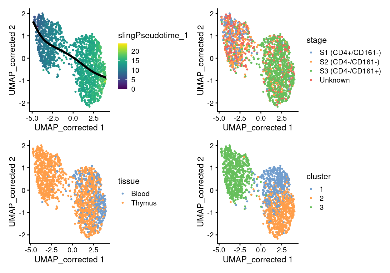
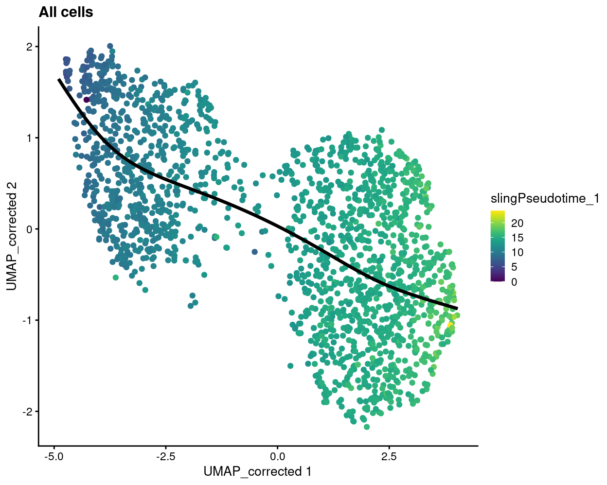
plotReducedDim(
  sce,
  dimred = "UMAP_corrected",
  colour_by = "slingPseudotime_1",
  point_alpha = 1,
  point_size = 0.5) +
  geom_path(data = embedded, aes(x = Dim.1, y = Dim.2), size = 1.2) +
  plotReducedDim(
    sce,
    dimred = "UMAP_corrected",
    colour_by = "stage",
    point_alpha = 1,
    point_size = 0.5) +
  plotReducedDim(
    sce,
    dimred = "UMAP_corrected",
    colour_by = "tissue",
    point_alpha = 1,
    point_size = 0.5) +
  plotReducedDim(
    sce,
    dimred = "UMAP_corrected",
    colour_by = "cluster",
    point_alpha = 1,
    point_size = 0.5) +
  plot_layout(ncol = 2)
Changes along a trajectory
We only test genes that are detected in at least 10 cells (\(n\) = 14,256).
We use methods from the TSCAN R/Bioconductor package. This is a simple method of testing for significant differences with respect to pseudotime, based on fitting linear models with a spline basis matrix.
Show code
library(TSCAN)
pseudo <- testPseudotime(
  sce_pseudo,
  pseudotime = sce_pseudo$slingPseudotime_1,
  block = sce_pseudo$plate_number)
pseudo <- pseudo[order(pseudo$p.value), ]

pseudotime_degs <- list(
  up_at_start =
    sapply(
      rowData(
        sce[rownames(pseudo[pseudo$FDR < 0.05 & pseudo$logFC < 0, ]), ])$NCBI.ENTREZID,
      "[[",
      1),
  up_at_end = sapply(
    rowData(
      sce[rownames(pseudo[pseudo$FDR < 0.05 & pseudo$logFC > 0, ]), ])$NCBI.ENTREZID,
    "[[",
    1))
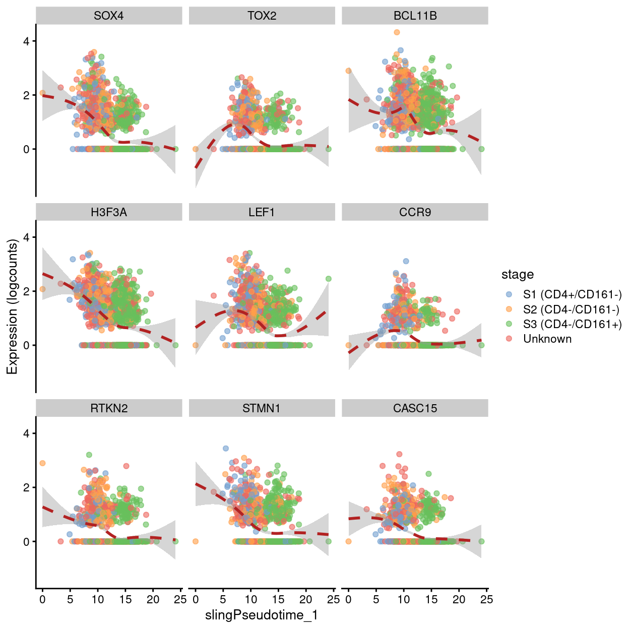
There are 707 and 381 genes that are significantly upregulated at the
start and end of the trajectory, respectively. CSV files of the results
are available from output/trajectory/.
Examples of genes upregulated at the beginning of pseudotime.
Show code
up.right <- pseudo[pseudo$logFC < 0, ]
best <- head(rownames(up.right), 9)
plotExpression(
  sce,
  features = best,
  x = "slingPseudotime_1",
  colour_by = "stage",
  show_smooth = TRUE,
  ncol = 3)
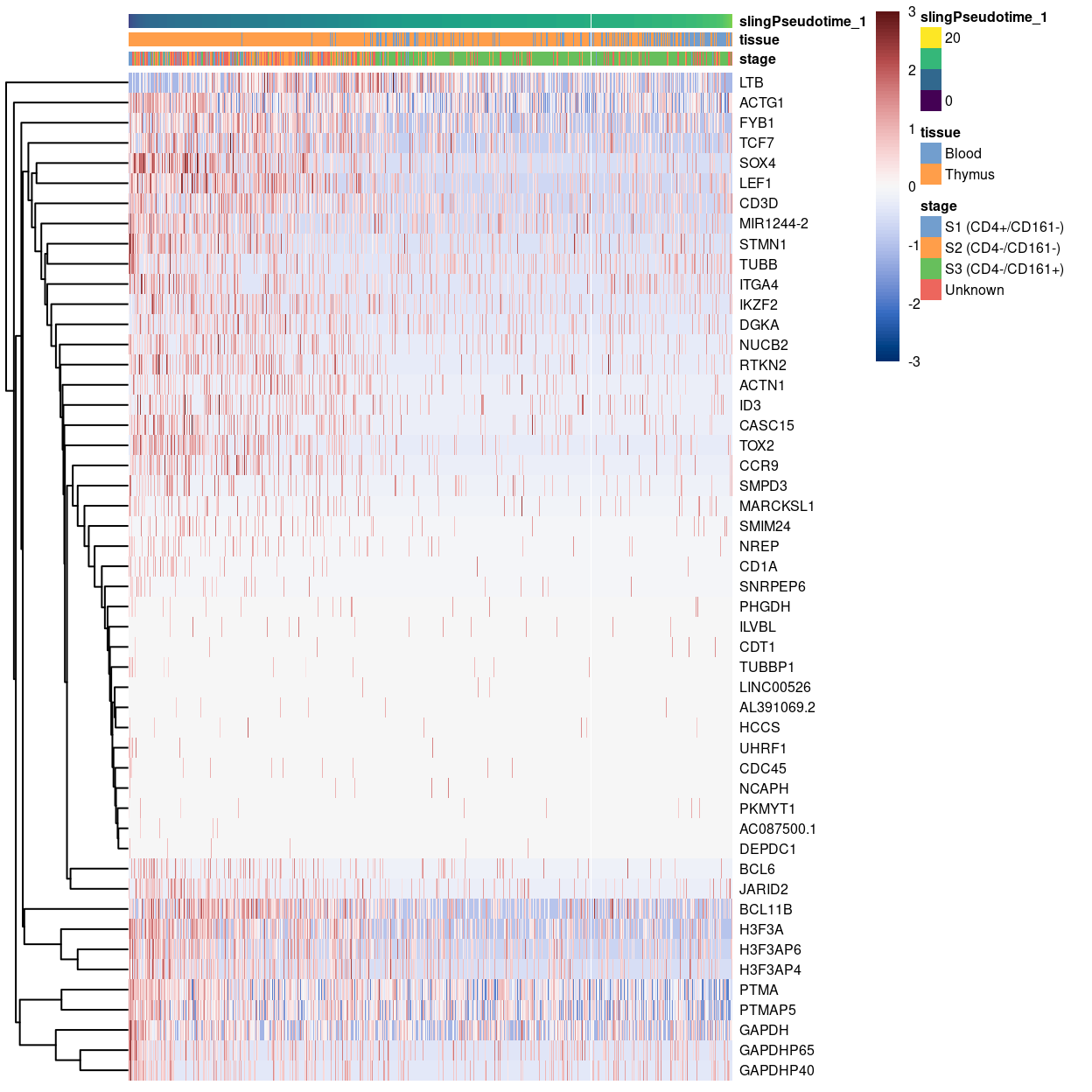
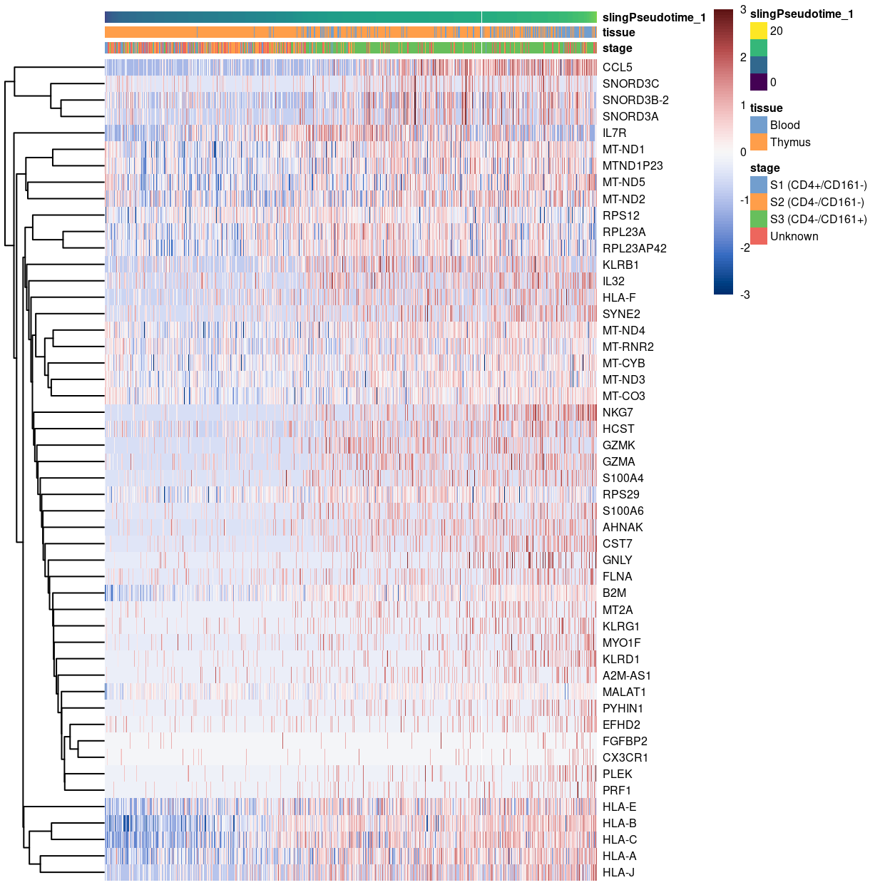
Heatmap of some genes upregulated at the beginning of pseudotime.
Show code
plotHeatmap(
  sce,
  order_columns_by = "slingPseudotime_1",
  colour_columns_by = c("stage", "tissue"),
  features = head(rownames(up.right), 50),
  center = TRUE,
  symmetric = TRUE,
  zlim = c(-3, 3),
  color = hcl.colors(101, "Blue-Red 3"),
  fontsize = 6)
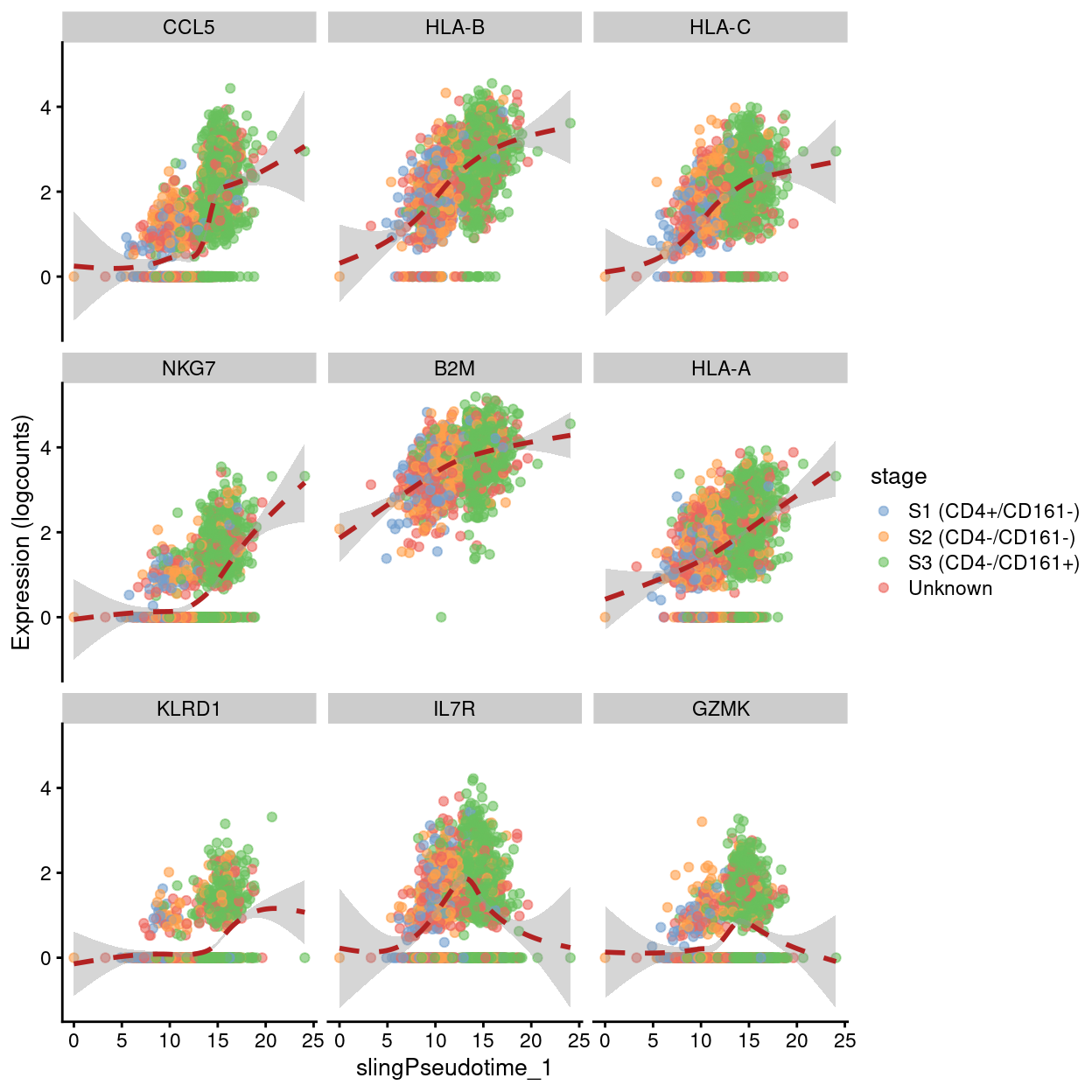
Examples of genes upregulated at the end of pseudotime.
Show code
up.right <- pseudo[pseudo$logFC > 0,]
best <- head(rownames(up.right), 9)
plotExpression(
  sce,
  features = best,
  x = "slingPseudotime_1",
  colour_by = "stage",
  show_smooth = TRUE,
  ncol = 3)
Heatmap of some genes upregulated at the end of pseudotime.
Show code
plotHeatmap(
  sce,
  order_columns_by = "slingPseudotime_1",
  colour_columns_by = c("stage", "tissue"),
  features = head(rownames(up.right), 50),
  center = TRUE,
  symmetric = TRUE,
  zlim = c(-3, 3),
  color = hcl.colors(101, "Blue-Red 3"),
  fontsize = 6)
Gene set testing
We use the TSCAN results and seek to identify gene sets that are differentially expressed with respect to the trajectory.
goana
We use the goana() function from the limma
R/Bioconductor package to test for over-representation of gene ontology
(GO) terms in each of the up_at_start and
up_at_end DEG lists.
CSV files of the results are available from output/trajectory/. An
example of the results are shown below, here ordered by
P.up_at_end to highlight GO terms that are enriched in the
up_at_end DEG list.
Show code
topGO(go, sort = "up_at_end") %>%
  knitr::kable(
    caption = '`goana()` produces a table with a row for each GO term and the following columns: **Term** (GO term); **Ont** (ontology that the GO term belongs to. Possible values are "BP", "CC" and "MF"); **N** (number of genes in the GO term); **up_at_start** (number of `up_at_start`-regulated differentially expressed genes); **up_at_end** (number of `up_at_end`-regulated differentially expressed genes); **P.up_at_start** (p-value for over-representation of GO term in `up_at_start`-regulated genes); **P.up_at_end** (p-value for over-representation of GO term in `up_at_end`-regulated genes)')
| Term | Ont | N | up_at_start | up_at_end | P.up_at_start | P.up_at_end | |
|---|---|---|---|---|---|---|---|
| GO:0002376 | immune system process | BP | 3287 | 112 | 117 | 0.0000123 | 0 |
| GO:0044419 | interspecies interaction between organisms | BP | 2250 | 86 | 93 | 0.0000023 | 0 |
| GO:0034097 | response to cytokine | BP | 1227 | 44 | 65 | 0.0029124 | 0 |
| GO:0006955 | immune response | BP | 2306 | 75 | 90 | 0.0016715 | 0 |
| GO:0071345 | cellular response to cytokine stimulus | BP | 1136 | 39 | 61 | 0.0098810 | 0 |
| GO:0009607 | response to biotic stimulus | BP | 1625 | 36 | 70 | 0.6444120 | 0 |
| GO:0019221 | cytokine-mediated signaling pathway | BP | 808 | 16 | 47 | 0.7788830 | 0 |
| GO:0051707 | response to other organism | BP | 1591 | 36 | 67 | 0.5928821 | 0 |
| GO:0043207 | response to external biotic stimulus | BP | 1593 | 36 | 67 | 0.5959871 | 0 |
| GO:0016032 | viral process | BP | 924 | 60 | 48 | 0.0000000 | 0 |
| GO:0006950 | response to stress | BP | 4162 | 116 | 116 | 0.0169229 | 0 |
| GO:0098542 | defense response to other organism | BP | 1213 | 27 | 55 | 0.6211128 | 0 |
| GO:0044403 | symbiotic process | BP | 983 | 62 | 49 | 0.0000000 | 0 |
| GO:0002252 | immune effector process | BP | 1299 | 43 | 57 | 0.0125215 | 0 |
| GO:0006952 | defense response | BP | 1824 | 39 | 69 | 0.7329622 | 0 |
| GO:0002682 | regulation of immune system process | BP | 1646 | 65 | 64 | 0.0000176 | 0 |
| GO:0045087 | innate immune response | BP | 996 | 25 | 48 | 0.3750108 | 0 |
| GO:0006614 | SRP-dependent cotranslational protein targeting to membrane | BP | 105 | 26 | 17 | 0.0000000 | 0 |
| GO:0006613 | cotranslational protein targeting to membrane | BP | 109 | 26 | 17 | 0.0000000 | 0 |
| GO:0022626 | cytosolic ribosome | CC | 110 | 25 | 17 | 0.0000000 | 0 |
kegga
We use the kegga() function from the limma
R/Bioconductor package to test for over-representation of KEGG pathways
in each of the up_at_start and up_at_end DEG
lists.
CSV files of the results are available from output/trajectory/. An
example of the results are shown below, here ordered by
P.up_at_end to highlight GO terms that are enriched in the
up_at_end DEG list.
Show code
topKEGG(kegg, sort = "up_at_end") %>%
  knitr::kable(
    caption = '`kegga()` produces a table with a row for each KEGG pathway ID and the following columns: **Pathway** (KEGG pathway); **N** (number of genes in the GO term);; **up_at_start** (number of `up_at_start`-regulated differentially expressed genes); **up_at_end** (number of `up_at_end`-regulated differentially expressed genes); **P.up_at_start** (p-value for over-representation of KEGG pathway in `up_at_start`-regulated genes); **P.up_at_end** (p-value for over-representation of KEGG pathway in `up_at_end`-regulated genes)')
| Pathway | N | up_at_start | up_at_end | P.up_at_start | P.up_at_end | |
|---|---|---|---|---|---|---|
| path:hsa03010 | Ribosome | 167 | 25 | 18 | 0.0000000 | 0.0000000 |
| path:hsa05332 | Graft-versus-host disease | 42 | 0 | 10 | 1.0000000 | 0.0000000 |
| path:hsa05171 | Coronavirus disease - COVID-19 | 232 | 27 | 20 | 0.0000000 | 0.0000000 |
| path:hsa04612 | Antigen processing and presentation | 78 | 0 | 11 | 1.0000000 | 0.0000003 |
| path:hsa04218 | Cellular senescence | 156 | 8 | 15 | 0.0836954 | 0.0000003 |
| path:hsa05330 | Allograft rejection | 38 | 0 | 8 | 1.0000000 | 0.0000005 |
| path:hsa04940 | Type I diabetes mellitus | 43 | 0 | 8 | 1.0000000 | 0.0000013 |
| path:hsa04650 | Natural killer cell mediated cytotoxicity | 132 | 4 | 13 | 0.5363094 | 0.0000014 |
| path:hsa05166 | Human T-cell leukemia virus 1 infection | 222 | 15 | 16 | 0.0019790 | 0.0000056 |
| path:hsa05163 | Human cytomegalovirus infection | 225 | 4 | 16 | 0.8967277 | 0.0000066 |
| path:hsa05320 | Autoimmune thyroid disease | 53 | 0 | 8 | 1.0000000 | 0.0000070 |
| path:hsa05169 | Epstein-Barr virus infection | 202 | 9 | 15 | 0.1328962 | 0.0000077 |
| path:hsa05416 | Viral myocarditis | 60 | 4 | 8 | 0.0957553 | 0.0000179 |
| path:hsa00190 | Oxidative phosphorylation | 134 | 12 | 11 | 0.0004963 | 0.0000532 |
| path:hsa05170 | Human immunodeficiency virus 1 infection | 212 | 10 | 14 | 0.0888054 | 0.0000581 |
| path:hsa04623 | Cytosolic DNA-sensing pathway | 75 | 0 | 8 | 1.0000000 | 0.0000923 |
| path:hsa04061 | Viral protein interaction with cytokine and cytokine receptor | 100 | 2 | 9 | 0.7918348 | 0.0001278 |
| path:hsa05167 | Kaposi sarcoma-associated herpesvirus infection | 194 | 6 | 12 | 0.4956586 | 0.0003651 |
| path:hsa05208 | Chemical carcinogenesis - reactive oxygen species | 223 | 14 | 13 | 0.0053522 | 0.0003698 |
| path:hsa04714 | Thermogenesis | 232 | 14 | 13 | 0.0075242 | 0.0005400 |
camera
We use the cameraPR() function1
from the limma
R/Bioconductor package to test whether a set of genes is highly ranked
relative to other genes in terms of differential expression, accounting
for inter-gene correlation. Specifically, we test using gene sets from
MSigDB,
namely:
- H: hallmark gene sets are coherently expressed signatures derived by aggregating many MSigDB gene sets to represent well-defined biological states or processes.
- C2: curated gene sets from online pathway databases, publications in PubMed, and knowledge of domain experts.
- C7: immunologic signature gene sets represent cell states and perturbations within the immune system.
Show code
# NOTE: Using BiocFileCache to avoid re-downloading these gene sets everytime
#       the report is rendered.
library(BiocFileCache)
bfc <- BiocFileCache()
# NOTE: Creating list of gene sets in this slightly convoluted way so that each
#       gene set name is prepended by its origin (e.g. H, C2, or C7).
msigdb <- do.call(
  c,
  list(
    H = readRDS(
      bfcrpath(
        bfc,
        "http://bioinf.wehi.edu.au/MSigDB/v7.1/Hs.h.all.v7.1.entrez.rds")),
    C2 = readRDS(
      bfcrpath(
        bfc,
        "http://bioinf.wehi.edu.au/MSigDB/v7.1/Hs.c2.all.v7.1.entrez.rds")),
    C7 = readRDS(
      bfcrpath(
        bfc,
        "http://bioinf.wehi.edu.au/MSigDB/v7.1/Hs.c7.all.v7.1.entrez.rds"))))

# Using the signed Z-score as the test statistic.
pseudo$statistic <- qnorm(pseudo$p.value / 2, lower.tail = FALSE) *
  sign(pseudo$logFC)
pseudo$ENTREZID <- sapply(
  rowData(sce[rownames(pseudo), ])$NCBI.ENTREZID,
  "[[",
  1)
y_idx <- ids2indices(msigdb, id = pseudo$ENTREZID)
cam <- cameraPR(
  statistic = setNames(pseudo$statistic, pseudo$ENTREZID),
  index = y_idx,
  use.ranks = FALSE)

gzout <- gzfile(
  description = file.path(outdir, "TSCAN_results.camera.csv.gz"),
  open = "wb")
write.csv(
  cam,
  gzout,
  row.names = TRUE)
close(gzout)
CSV files of the results are available from output/trajectory/. An
example of the results are shown below, here filtered to highlight those
gene sets with Direction = Up meaning
up_at_end.
Show code
head(cam[cam$Direction == "Up", ]) %>%
  knitr::kable(
    caption = '`camera()` produces a table with a row for each gene set (prepended by which MSigDB collection it comes from) and the following columns: **NGenes** (number of genes in set); **Direction** (direction of change, `Up` = `up_at_end` and `Down` = `up_at_start`); **PValue** (two-tailed p-value); **FDR** (Benjamini and Hochberg FDR adjusted p-value).')
| NGenes | Direction | PValue | FDR | |
|---|---|---|---|---|
| C2.REACTOME_ENDOSOMAL_VACUOLAR_PATHWAY | 9 | Up | 0 | 0 |
| C2.HAHTOLA_CTCL_PATHOGENESIS | 11 | Up | 0 | 0 |
| C2.KIM_LRRC3B_TARGETS | 26 | Up | 0 | 0 |
| C2.WUNDER_INFLAMMATORY_RESPONSE_AND_CHOLESTEROL_DN | 3 | Up | 0 | 0 |
| C2.HAHTOLA_SEZARY_SYNDROM_DN | 34 | Up | 0 | 0 |
| C2.KEGG_GRAFT_VERSUS_HOST_DISEASE | 25 | Up | 0 | 0 |
Visualisation
Show code
term <- "C2.REACTOME_INTERFERON_ALPHA_BETA_SIGNALING"
library(org.Hs.eg.db)
key <- msigdb[[term]]
tmp <- AnnotationDbi::select(
  org.Hs.eg.db,
  key = key,
  columns = "SYMBOL",
  keytype = "ENTREZID")
y_index <- ids2indices(msigdb[[term]], pseudo$ENTREZID)
We can visualise the expression of the genes in any given set using a ‘barcode plot’. Such figures are often included in publications.
Figure 1 gives an example showing the expression of genes in the C2.REACTOME_INTERFERON_ALPHA_BETA_SIGNALING MSigDB gene set.
Show code
barcodeplot(statistics = pseudo$statistic, index = y_index[[1]])
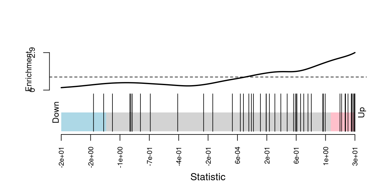
Figure 1: Barcode plot of genes in MSigDB set
C2.REACTOME_INTERFERON_ALPHA_BETA_SIGNALING. Genes are
represented by bars and are ranked from left to right by increasing
signed Wald statistic from the trajectory DE analysis. This forms the
barcode-like pattern. The line (or worm) above the barcode
shows the relative local enrichment of the vertical bars in each part of
the plot. The dotted horizontal line indicates neutral enrichment; the
worm above the dotted line shows enrichment while the worm below the
dotted line shows depletion.
Figures for paper
Note that exact figure numbers may change.
Show code
# Some useful colours
plate_number_colours <- setNames(
  unique(sce$colours$plate_number_colours),
  unique(names(sce$colours$plate_number_colours)))
plate_number_colours <- plate_number_colours[levels(sce$plate_number)]
tissue_colours <- setNames(
  unique(sce$colours$tissue_colours),
  unique(names(sce$colours$tissue_colours)))
tissue_colours <- tissue_colours[levels(sce$tissue)]
donor_colours <- setNames(
  unique(sce$colours$donor_colours),
  unique(names(sce$colours$donor_colours)))
donor_colours <- donor_colours[levels(sce$donor)]
stage_colours <- setNames(
  unique(sce$colours$stage_colours),
  unique(names(sce$colours$stage_colours)))
stage_colours <- stage_colours[levels(sce$stage)]
group_colours <- setNames(
  unique(sce$colours$group_colours),
  unique(names(sce$colours$group_colours)))
group_colours <- group_colours[levels(sce$group)]
cluster_colours <- setNames(
  unique(sce$colours$cluster_colours),
  unique(names(sce$colours$cluster_colours)))
cluster_colours <- cluster_colours[levels(sce$cluster)]
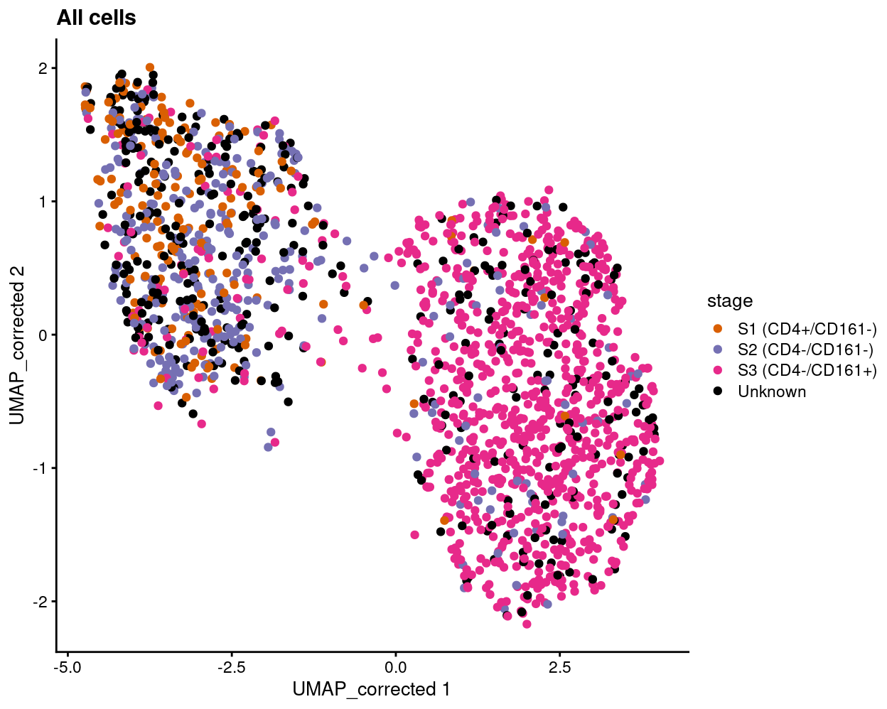
Figure 5
Show code
plotReducedDim(
  sce,
  "UMAP_corrected",
  colour_by = "stage",
  point_alpha = 1) +
  scale_colour_manual(values = stage_colours, name = "stage") +
  ggtitle("All cells")
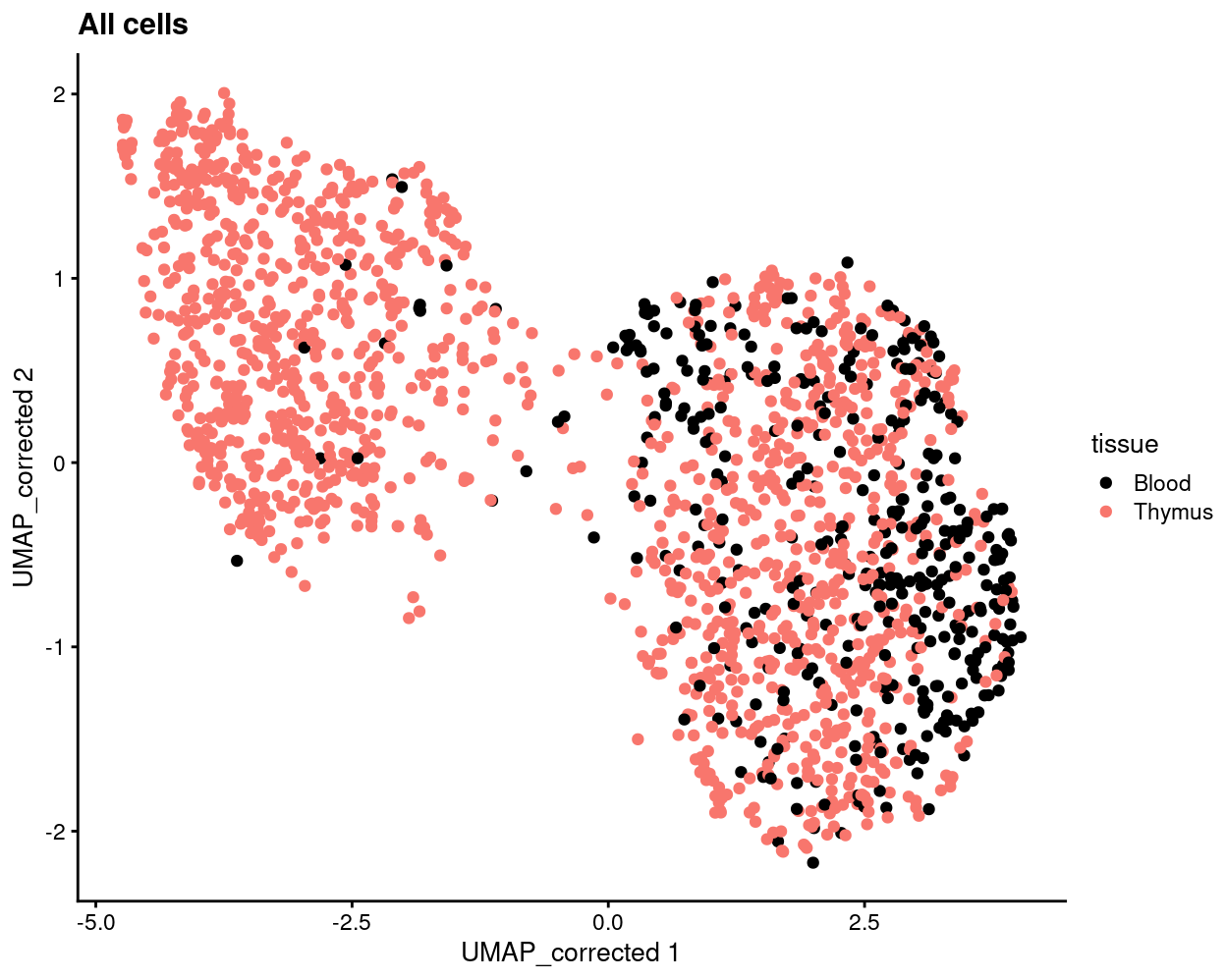
Show code
plotReducedDim(
  sce,
  "UMAP_corrected",
  colour_by = "tissue",
  point_alpha = 1) +
  scale_colour_manual(values = tissue_colours, name = "tissue") +
  ggtitle("All cells")
Show code
plotReducedDim(
  sce,
  dimred = "UMAP_corrected",
  colour_by = "slingPseudotime_1",
  point_alpha = 1) +
  geom_path(data = embedded, aes(x = Dim.1, y = Dim.2), size = 1.2) +
  ggtitle("All cells")
Show code
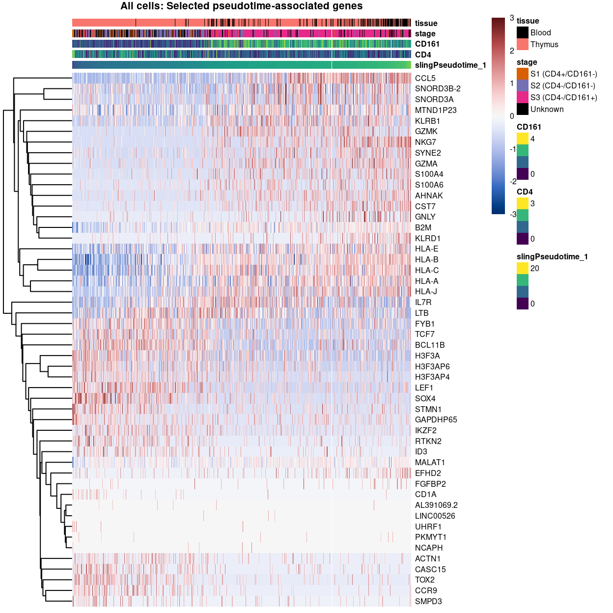
plotHeatmap(
  sce,
  order_columns_by = "slingPseudotime_1",
  colour_columns_by = c("slingPseudotime_1", "CD4", "CD161", "stage", "tissue"),
  features = c(
    head(
      setdiff(
        rownames(pseudo[pseudo$FDR < 0.05 & pseudo$logFC < 0, ]),
        mito_set),
      25),
    head(
      setdiff(
        rownames(pseudo[pseudo$FDR < 0.05 & pseudo$logFC > 0, ]),
        mito_set),
      25)),
  center = TRUE,
  symmetric = TRUE,
  zlim = c(-3, 3),
  color = hcl.colors(101, "Blue-Red 3"),
  fontsize = 6,
  main = "All cells: Selected pseudotime-associated genes",
  column_annotation_colors = list(
    stage = stage_colours,
    tissue = tissue_colours))
Show code
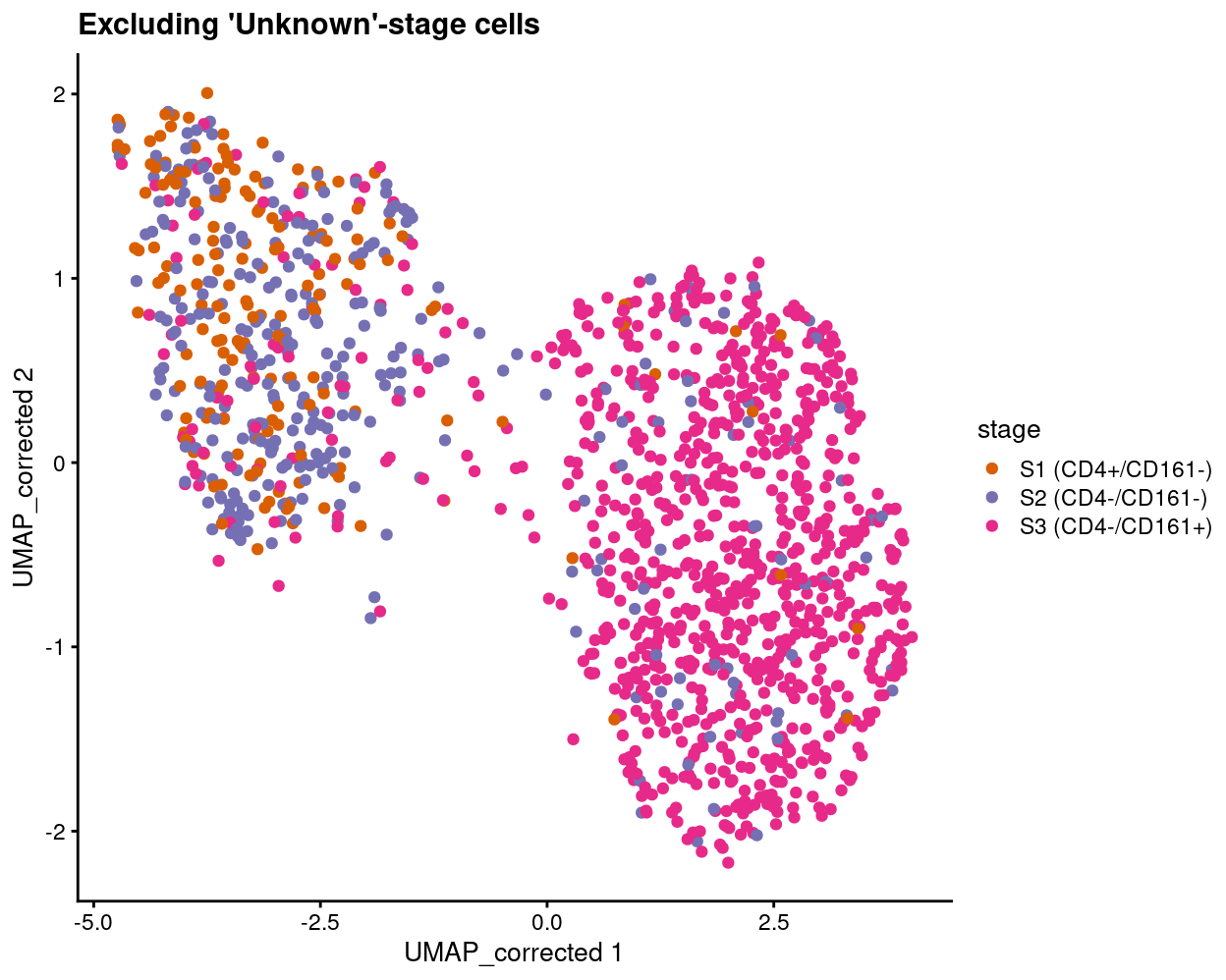
plotReducedDim(
sce[, sce$stage != "Unknown"],
"UMAP_corrected",
colour_by = "stage",
point_alpha = 1) +
scale_colour_manual(values = stage_colours, name = "stage") +
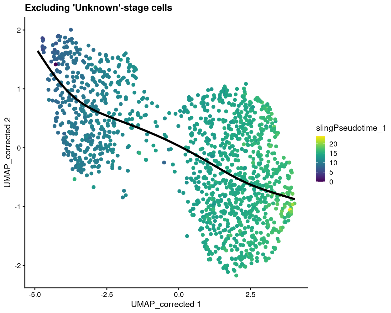
ggtitle("Excluding 'Unknown'-stage cells")
Show code
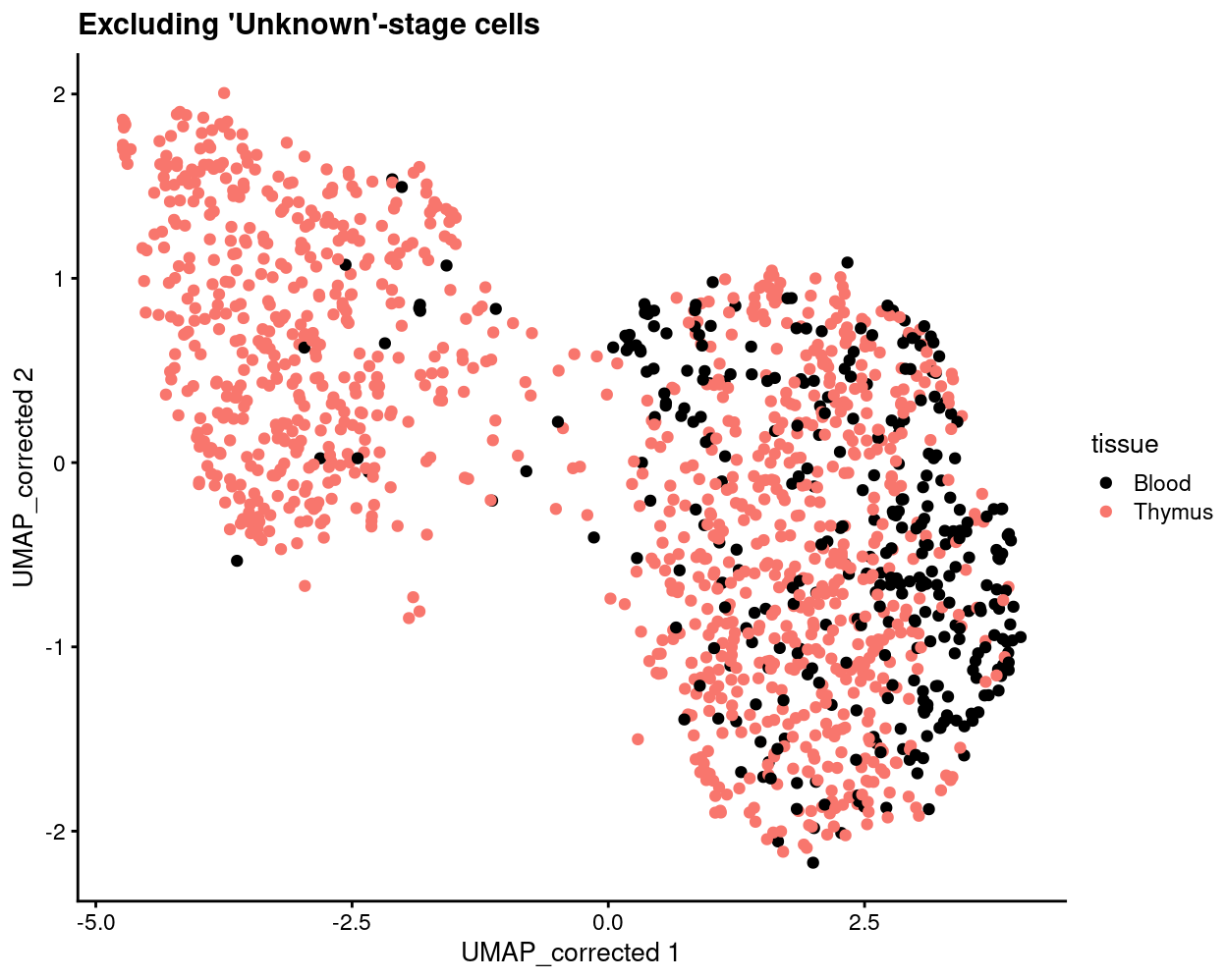
plotReducedDim(
  sce[, sce$stage != "Unknown"],
  "UMAP_corrected",
  colour_by = "tissue",
  point_alpha = 1) +
  scale_colour_manual(values = tissue_colours, name = "tissue") +
  ggtitle("Excluding 'Unknown'-stage cells")
Show code
plotReducedDim(
  sce[, sce$stage != "Unknown"],
  dimred = "UMAP_corrected",
  colour_by = "slingPseudotime_1",
  point_alpha = 1) +
  geom_path(data = embedded, aes(x = Dim.1, y = Dim.2), size = 1.2) +
  ggtitle("Excluding 'Unknown'-stage cells")
Show code
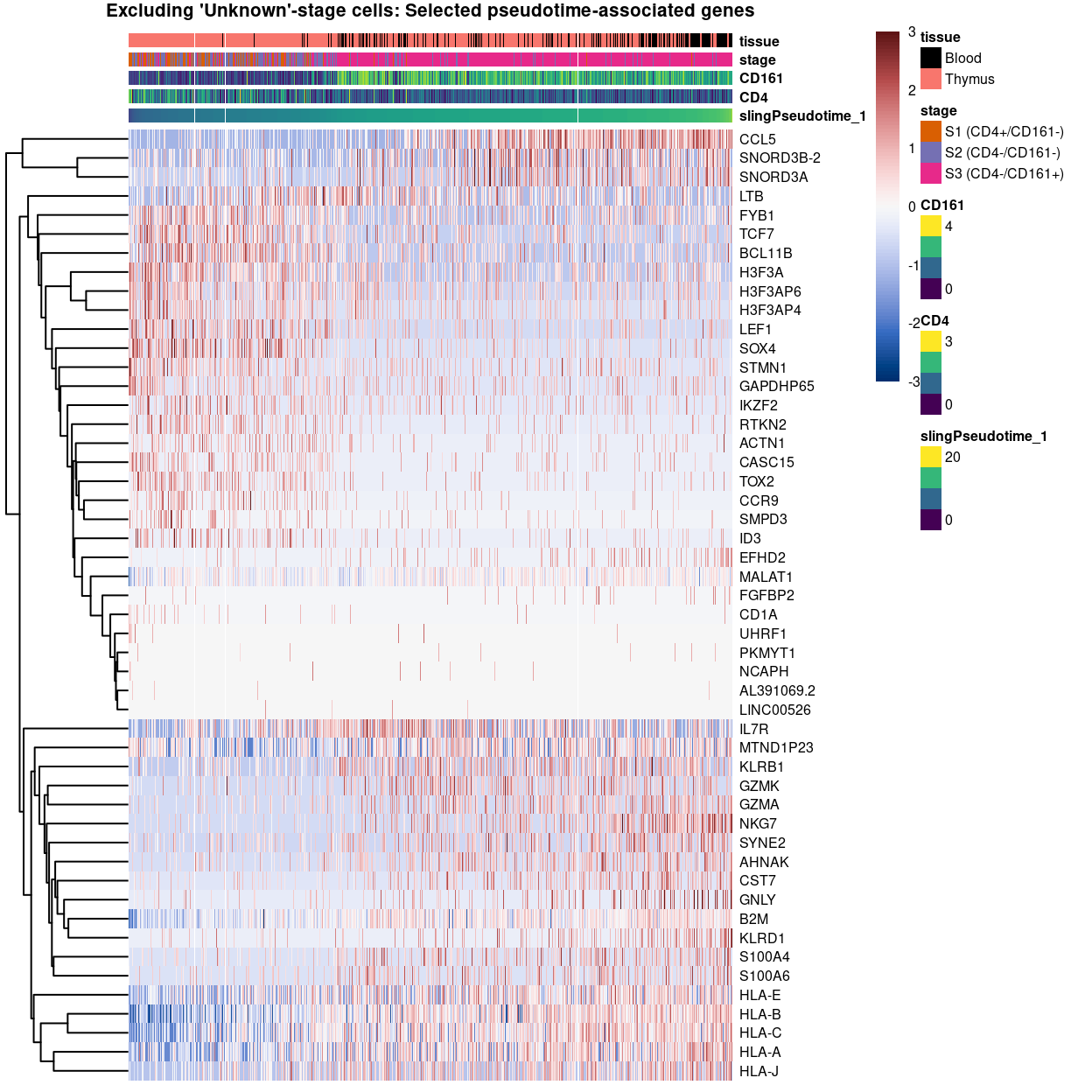
plotHeatmap(
  sce[, sce$stage != "Unknown"],
  order_columns_by = "slingPseudotime_1",
  colour_columns_by = c("slingPseudotime_1", "CD4", "CD161", "stage", "tissue"),
  features = c(
    head(
      setdiff(
        rownames(pseudo[pseudo$FDR < 0.05 & pseudo$logFC < 0, ]),
        mito_set),
      25),
    head(
      setdiff(
        rownames(pseudo[pseudo$FDR < 0.05 & pseudo$logFC > 0, ]),
        mito_set),
      25)),
  center = TRUE,
  symmetric = TRUE,
  zlim = c(-3, 3),
  color = hcl.colors(101, "Blue-Red 3"),
  fontsize = 6,
  main = "Excluding 'Unknown'-stage cells: Selected pseudotime-associated genes",
  column_annotation_colors = list(
    stage = stage_colours[levels(factor(sce[, sce$stage != "Unknown"]$stage))],
    tissue = tissue_colours))
DEG heatmaps
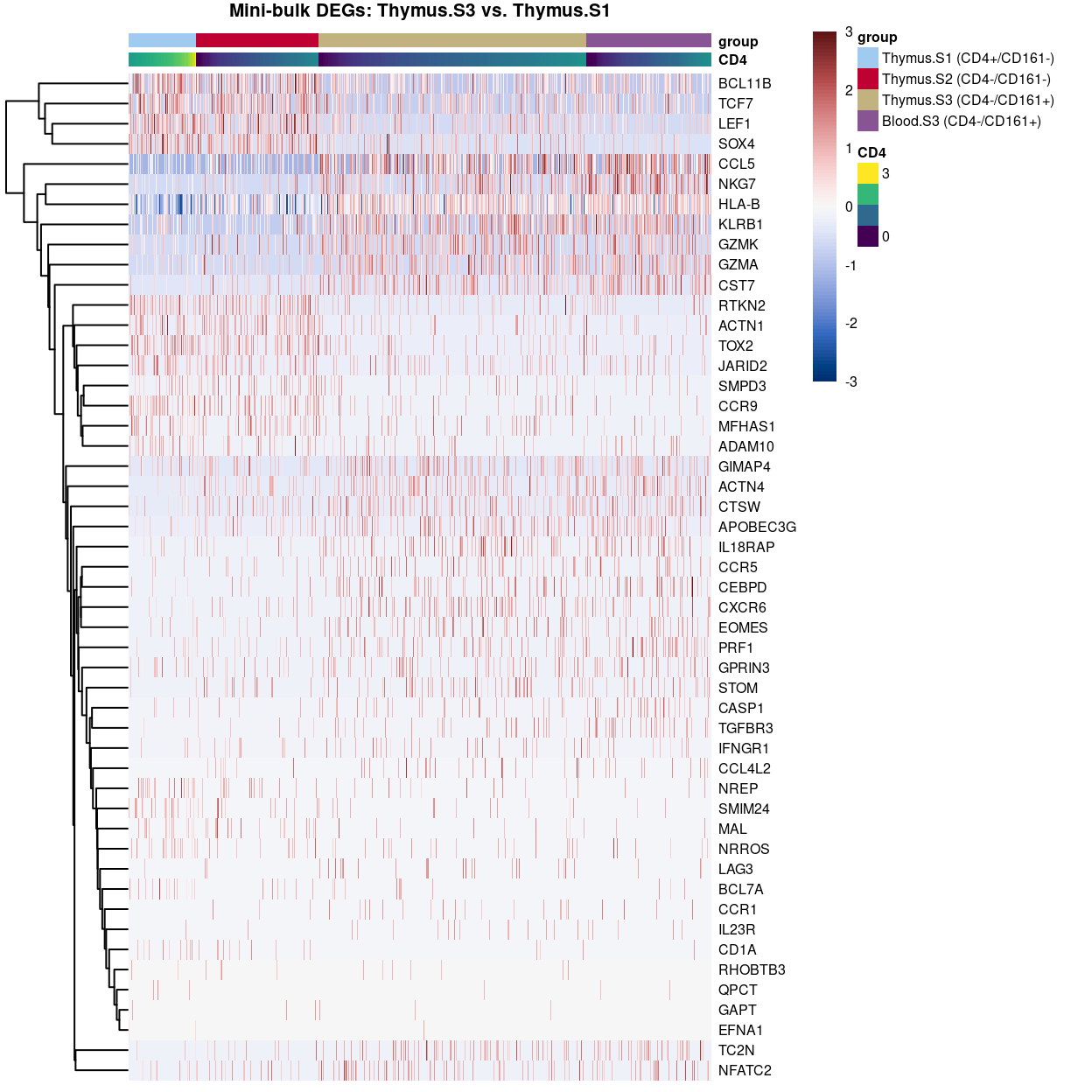
Heatmaps sorted by CD4 and CD161 FACS expression “showing the DEGs across the gamma delta T cell stages ordered by decreasing either CD4 or KLRB1.” This is an example, but, as I explained to Dan, I don’t think these are very useful plots.
Show code
tmp <- sce[
  ,
  sce$group %in%
    c("Thymus.S1 (CD4+/CD161-)",
      "Thymus.S2 (CD4-/CD161-)",
      "Thymus.S3 (CD4-/CD161+)",
      "Blood.S3 (CD4-/CD161+)")]
tmp$group <- factor(
  tmp$group,
  c("Thymus.S1 (CD4+/CD161-)",
    "Thymus.S2 (CD4-/CD161-)",
    "Thymus.S3 (CD4-/CD161+)",
    "Blood.S3 (CD4-/CD161+)"))

x <- read.csv(
  here(
    "output",
    "DEGs",
    "excluding_donors_1-3",
    "Thymus.S3_vs_Thymus.S1.aggregated_tech_reps.DEGs.csv.gz"))
Show code
plotHeatmap(
  tmp,
  order_columns_by = c("group", "CD4"),
  colour_columns_by = c("CD4", "group"),
  features = head(x[x$FDR < 0.05, "ENSEMBL.SYMBOL"], 50),
  center = TRUE,
  symmetric = TRUE,
  zlim = c(-3, 3),
  color = hcl.colors(101, "Blue-Red 3"),
  fontsize = 6,
  main = "Mini-bulk DEGs: Thymus.S3 vs. Thymus.S1",
  column_annotation_colors = list(group = group_colours[levels(tmp$group)]))
Show code
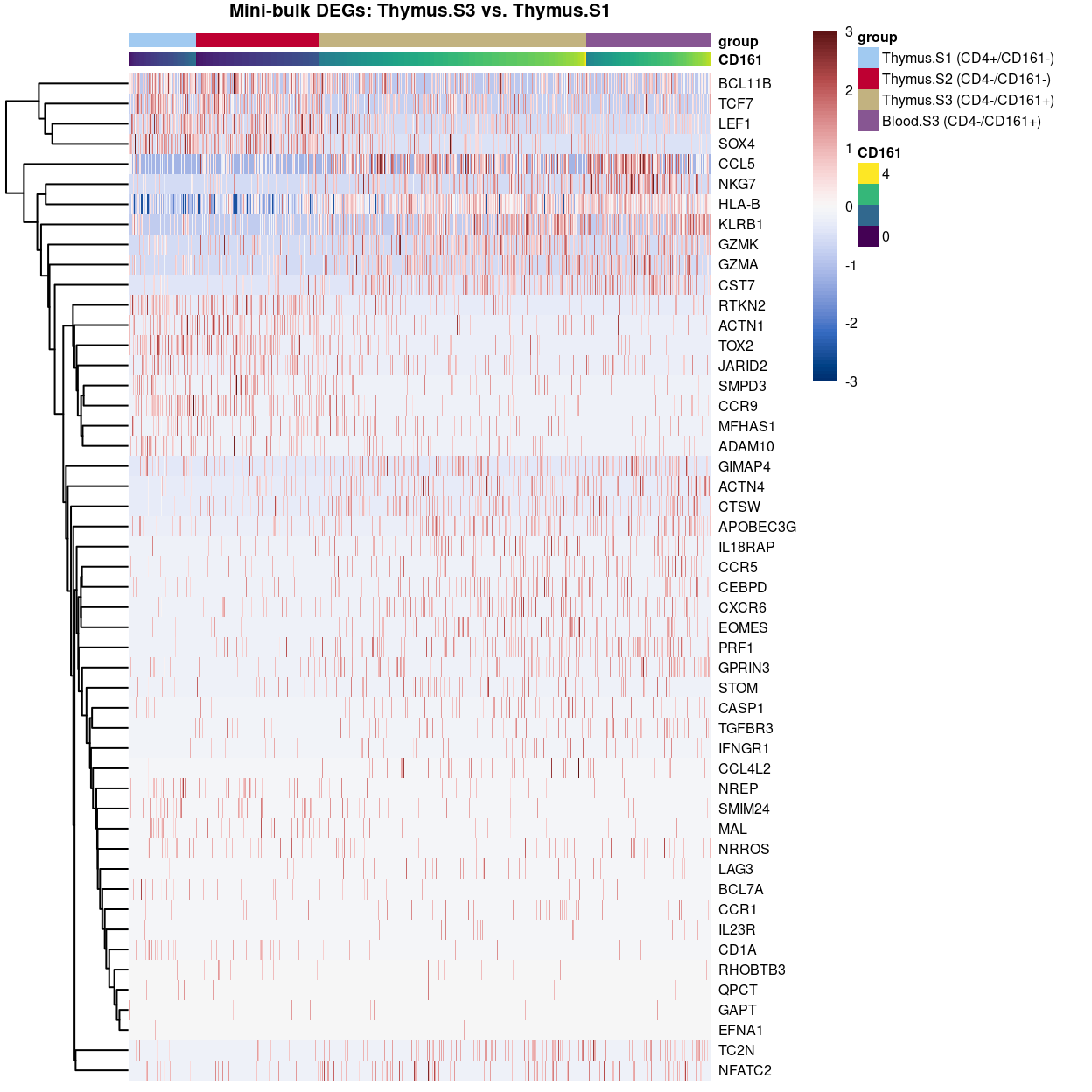
plotHeatmap(
  tmp,
  order_columns_by = c("group", "CD161"),
  colour_columns_by = c("CD161", "group"),
  features = head(x[x$FDR < 0.05, "ENSEMBL.SYMBOL"], 50),
  center = TRUE,
  symmetric = TRUE,
  zlim = c(-3, 3),
  color = hcl.colors(101, "Blue-Red 3"),
  fontsize = 6,
  main = "Mini-bulk DEGs: Thymus.S3 vs. Thymus.S1",
  column_annotation_colors = list(group = group_colours[levels(tmp$group)]))
Mock figure sent to Dan and co (2021-09-09)
Show code
dir.create(here("output/figures"))

p1 <- plotReducedDim(
  sce[, sce$stage != "Unknown"],
  "UMAP_corrected",
  colour_by = "stage",
  point_alpha = 1) +
  scale_colour_manual(values = stage_colours, name = "stage")
ggsave(here("output/figures/Fig5a.pdf"), p1, width = 6, height = 5)

p2 <- plotReducedDim(
  sce[, sce$stage != "Unknown"],
  "UMAP_corrected",
  colour_by = "tissue",
  point_alpha = 1) +
  scale_colour_manual(values = tissue_colours, name = "tissue")
ggsave(here("output/figures/Fig5b.pdf"), p2, width = 6, height = 5)

p3 <- plotReducedDim(
  sce[, sce$stage != "Unknown"],
  dimred = "UMAP_corrected",
  colour_by = "slingPseudotime_1",
  point_alpha = 1) +
  geom_path(data = embedded, aes(x = Dim.1, y = Dim.2), size = 1.2)
ggsave(here("output/figures/Fig5c.pdf"), p3, width = 6, height = 5)

p4 <- plotHeatmap(
  sce,
  order_columns_by = "slingPseudotime_1",
  colour_columns_by = c("slingPseudotime_1", "CD4", "CD161", "stage", "tissue"),
  features = c(
    head(
      setdiff(
        rownames(pseudo[pseudo$FDR < 0.05 & pseudo$logFC < 0, ]),
        mito_set),
      25),
    head(
      setdiff(
        rownames(pseudo[pseudo$FDR < 0.05 & pseudo$logFC > 0, ]),
        mito_set),
      25)),
  center = TRUE,
  symmetric = TRUE,
  zlim = c(-3, 3),
  color = hcl.colors(101, "Blue-Red 3"),
  fontsize = 6,
  main = "All cells: Selected pseudotime-associated genes",
  column_annotation_colors = list(
    stage = stage_colours,
    tissue = tissue_colours),
  silent = TRUE)
ggsave(here("output/figures/Fig5d.pdf"), p4$gtable, width = 6, height = 8)

p4a <- plotHeatmap(
  sce[, sce$stage != "Unknown"],
  order_columns_by = "slingPseudotime_1",
  colour_columns_by = c("slingPseudotime_1", "CD4", "CD161", "stage", "tissue"),
  features = c(
    head(
      setdiff(
        rownames(pseudo[pseudo$FDR < 0.05 & pseudo$logFC < 0, ]),
        mito_set),
      25),
    head(
      setdiff(
        rownames(pseudo[pseudo$FDR < 0.05 & pseudo$logFC > 0, ]),
        mito_set),
      25)),
  center = TRUE,
  symmetric = TRUE,
  zlim = c(-3, 3),
  color = hcl.colors(101, "Blue-Red 3"),
  fontsize = 6,
  main = "Excluding 'Unknown'-stage cells: Selected pseudotime-associated genes",
  column_annotation_colors = list(
    stage = stage_colours[levels(factor(sce[, sce$stage != "Unknown"]$stage))],
    tissue = tissue_colours),
  silent = TRUE)
ggsave(
  here("output/figures/Fig5d_alternative.pdf"),
  p4a$gtable,
  width = 6,
  height = 8)
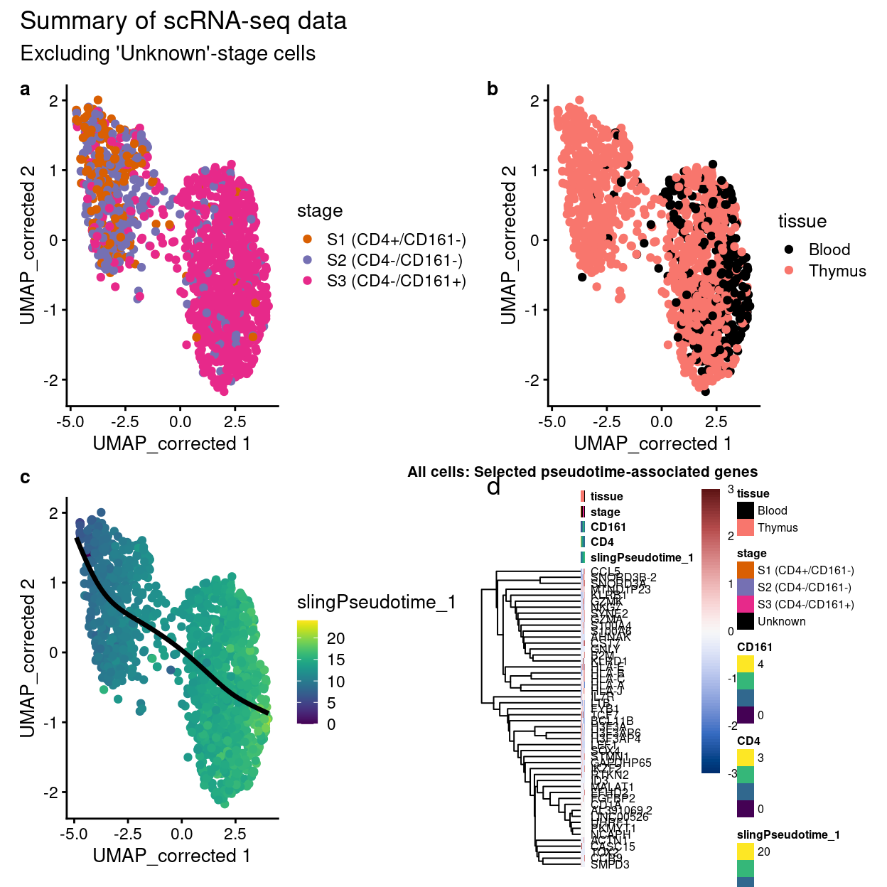
Initial proposal:
Show code
p1 + p2 + p3 + p4$gtable +
  plot_annotation(
    title = "Summary of scRNA-seq data",
    subtitle = "Excluding 'Unknown'-stage cells",
    tag_levels = "a")
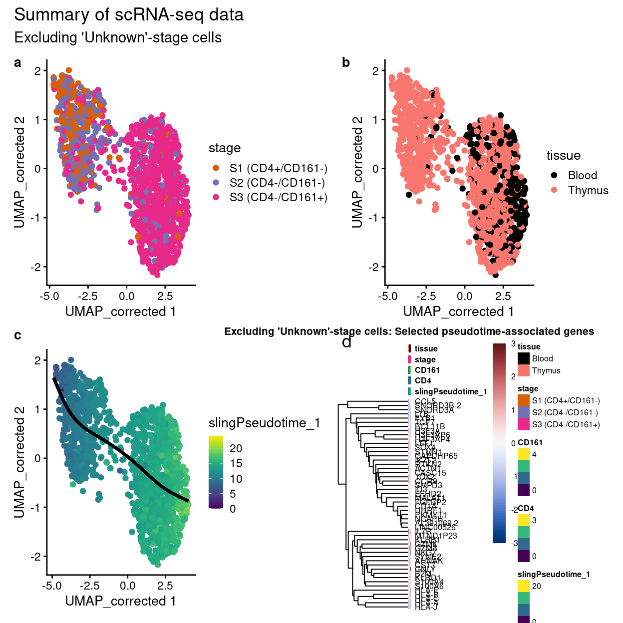
Alternative:
Show code
p1 + p2 + p3 + p4a$gtable +
  plot_annotation(
    title = "Summary of scRNA-seq data",
    subtitle = "Excluding 'Unknown'-stage cells",
    tag_levels = "a")
Additional information
The following are available on request:
- Full CSV tables of any data presented.
- PDF/PNG files of any static plots.
Session info
Show code
sessioninfo::session_info()
─ Session info ─────────────────────────────────────────────────────
 setting  value
 version  R version 4.0.5 (2021-03-31)
 os       CentOS Linux 7 (Core)
 system   x86_64, linux-gnu
 ui       X11
 language (EN)
 collate  en_US.UTF-8
 ctype    en_US.UTF-8
 tz       Australia/Melbourne
 date     2023-02-22

─ Packages ─────────────────────────────────────────────────────────
 ! package              * version  date       lib source
 P AnnotationDbi        * 1.52.0   2020-10-27 [?] Bioconductor
 P ape                    5.5      2021-04-25 [?] CRAN (R 4.0.5)
 P assertthat             0.2.1    2019-03-21 [?] CRAN (R 4.0.5)
 P beachmat               2.6.4    2020-12-20 [?] Bioconductor
 P beeswarm               0.3.1    2021-03-07 [?] CRAN (R 4.0.5)
 P Biobase              * 2.50.0   2020-10-27 [?] Bioconductor
 P BiocFileCache        * 1.14.0   2020-10-27 [?] Bioconductor
 P BiocGenerics         * 0.36.0   2020-10-27 [?] Bioconductor
 P BiocManager            1.30.12  2021-03-28 [?] CRAN (R 4.0.5)
 P BiocNeighbors          1.8.2    2020-12-07 [?] Bioconductor
 P BiocParallel           1.24.1   2020-11-06 [?] Bioconductor
 P BiocSingular           1.6.0    2020-10-27 [?] Bioconductor
 P BiocStyle              2.18.1   2020-11-24 [?] Bioconductor
 P bit                    4.0.4    2020-08-04 [?] CRAN (R 4.0.5)
 P bit64                  4.0.5    2020-08-30 [?] CRAN (R 4.0.5)
 P bitops                 1.0-6    2013-08-17 [?] CRAN (R 4.0.5)
 P blob                   1.2.1    2020-01-20 [?] CRAN (R 4.0.5)
 P bluster                1.0.0    2020-10-27 [?] Bioconductor
 P bslib                  0.4.0    2022-07-16 [?] CRAN (R 4.0.5)
 P cachem                 1.0.4    2021-02-13 [?] CRAN (R 4.0.5)
 P caTools                1.18.2   2021-03-28 [?] CRAN (R 4.0.5)
 P cli                    2.4.0    2021-04-05 [?] CRAN (R 4.0.5)
 P colorspace             2.0-0    2020-11-11 [?] CRAN (R 4.0.5)
 P combinat               0.0-8    2012-10-29 [?] CRAN (R 4.0.5)
 P cowplot                1.1.1    2020-12-30 [?] CRAN (R 4.0.5)
 P crayon                 1.4.1    2021-02-08 [?] CRAN (R 4.0.5)
 P curl                   4.3      2019-12-02 [?] CRAN (R 4.0.5)
 P DBI                    1.1.1    2021-01-15 [?] CRAN (R 4.0.5)
 P dbplyr               * 2.1.0    2021-02-03 [?] CRAN (R 4.0.5)
 P DelayedArray           0.16.3   2021-03-24 [?] Bioconductor
 P DelayedMatrixStats     1.12.3   2021-02-03 [?] Bioconductor
 P digest                 0.6.27   2020-10-24 [?] CRAN (R 4.0.5)
 P distill                1.2      2021-01-13 [?] CRAN (R 4.0.5)
 P downlit                0.2.1    2020-11-04 [?] CRAN (R 4.0.5)
 P dplyr                  1.0.5    2021-03-05 [?] CRAN (R 4.0.5)
 P dqrng                  0.2.1    2019-05-17 [?] CRAN (R 4.0.5)
 P edgeR                  3.32.1   2021-01-14 [?] Bioconductor
 P ellipsis               0.3.1    2020-05-15 [?] CRAN (R 4.0.5)
 P evaluate               0.14     2019-05-28 [?] CRAN (R 4.0.5)
 P fansi                  0.4.2    2021-01-15 [?] CRAN (R 4.0.5)
 P farver                 2.1.0    2021-02-28 [?] CRAN (R 4.0.5)
 P fastICA                1.2-2    2019-07-08 [?] CRAN (R 4.0.5)
 P fastmap                1.1.0    2021-01-25 [?] CRAN (R 4.0.5)
 P generics               0.1.0    2020-10-31 [?] CRAN (R 4.0.5)
 P GenomeInfoDb         * 1.26.4   2021-03-10 [?] Bioconductor
 P GenomeInfoDbData       1.2.4    2023-02-21 [?] Bioconductor
 P GenomicRanges        * 1.42.0   2020-10-27 [?] Bioconductor
 P ggbeeswarm             0.6.0    2017-08-07 [?] CRAN (R 4.0.5)
 P ggplot2              * 3.3.3    2020-12-30 [?] CRAN (R 4.0.5)
 P glue                   1.4.2    2020-08-27 [?] CRAN (R 4.0.5)
 P GO.db                  3.12.1   2023-02-21 [?] Bioconductor
 P gplots                 3.1.3    2022-04-25 [?] CRAN (R 4.0.5)
 P gridExtra              2.3      2017-09-09 [?] CRAN (R 4.0.5)
 P gtable                 0.3.0    2019-03-25 [?] CRAN (R 4.0.5)
   gtools                 3.9.2    2021-06-06 [2] CRAN (R 4.0.5)
 P here                 * 1.0.1    2020-12-13 [?] CRAN (R 4.0.5)
 P highr                  0.9      2021-04-16 [?] CRAN (R 4.0.5)
 P htmltools              0.5.3    2022-07-18 [?] CRAN (R 4.0.5)
 P httpuv                 1.5.5    2021-01-13 [?] CRAN (R 4.0.5)
 P httr                   1.4.2    2020-07-20 [?] CRAN (R 4.0.5)
 P igraph                 1.2.6    2020-10-06 [?] CRAN (R 4.0.5)
 P IRanges              * 2.24.1   2020-12-12 [?] Bioconductor
 P irlba                  2.3.3    2019-02-05 [?] CRAN (R 4.0.5)
 P jquerylib              0.1.3    2020-12-17 [?] CRAN (R 4.0.5)
 P jsonlite               1.7.2    2020-12-09 [?] CRAN (R 4.0.5)
 P KernSmooth             2.23-17  2020-04-26 [?] CRAN (R 4.0.3)
 P knitr                  1.33     2021-04-24 [?] CRAN (R 4.0.5)
 P labeling               0.4.2    2020-10-20 [?] CRAN (R 4.0.5)
 P later                  1.1.0.1  2020-06-05 [?] CRAN (R 4.0.5)
 P lattice                0.20-41  2020-04-02 [?] CRAN (R 4.0.3)
 P lifecycle              1.0.0    2021-02-15 [?] CRAN (R 4.0.5)
 P limma                * 3.46.0   2020-10-27 [?] Bioconductor
 P locfit                 1.5-9.4  2020-03-25 [?] CRAN (R 4.0.5)
 P magrittr               2.0.1    2020-11-17 [?] CRAN (R 4.0.5)
 P Matrix                 1.2-18   2019-11-27 [?] CRAN (R 4.0.3)
 P MatrixGenerics       * 1.2.1    2021-01-30 [?] Bioconductor
 P matrixStats          * 0.58.0   2021-01-29 [?] CRAN (R 4.0.5)
 P mclust                 5.4.7    2020-11-20 [?] CRAN (R 4.0.5)
 P memoise                2.0.0    2021-01-26 [?] CRAN (R 4.0.5)
 P mgcv                   1.8-33   2020-08-27 [?] CRAN (R 4.0.3)
 P mime                   0.11     2021-06-23 [?] CRAN (R 4.0.5)
 P msigdbr              * 7.2.1    2020-10-02 [?] CRAN (R 4.0.5)
 P munsell                0.5.0    2018-06-12 [?] CRAN (R 4.0.5)
 P nlme                   3.1-149  2020-08-23 [?] CRAN (R 4.0.3)
 P org.Hs.eg.db         * 3.12.0   2023-02-21 [?] Bioconductor
 P patchwork            * 1.1.1    2020-12-17 [?] CRAN (R 4.0.5)
 P pheatmap               1.0.12   2019-01-04 [?] CRAN (R 4.0.5)
 P pillar                 1.5.1    2021-03-05 [?] CRAN (R 4.0.5)
 P pkgconfig              2.0.3    2019-09-22 [?] CRAN (R 4.0.5)
 P plyr                   1.8.6    2020-03-03 [?] CRAN (R 4.0.5)
 P princurve            * 2.1.6    2021-01-18 [?] CRAN (R 4.0.5)
 P promises               1.2.0.1  2021-02-11 [?] CRAN (R 4.0.5)
 P purrr                  0.3.4    2020-04-17 [?] CRAN (R 4.0.5)
 P R6                     2.5.0    2020-10-28 [?] CRAN (R 4.0.5)
 P rappdirs               0.3.3    2021-01-31 [?] CRAN (R 4.0.5)
 P RColorBrewer           1.1-2    2014-12-07 [?] CRAN (R 4.0.5)
 P Rcpp                   1.0.6    2021-01-15 [?] CRAN (R 4.0.5)
 P RCurl                  1.98-1.3 2021-03-16 [?] CRAN (R 4.0.5)
 P rlang                  0.4.11   2021-04-30 [?] CRAN (R 4.0.5)
 P rmarkdown              2.14     2022-04-25 [?] CRAN (R 4.0.5)
 P rprojroot              2.0.2    2020-11-15 [?] CRAN (R 4.0.5)
 P RSQLite                2.2.5    2021-03-27 [?] CRAN (R 4.0.5)
 P rsvd                   1.0.3    2020-02-17 [?] CRAN (R 4.0.5)
 P S4Vectors            * 0.28.1   2020-12-09 [?] Bioconductor
 P sass                   0.4.2    2022-07-16 [?] CRAN (R 4.0.5)
 P scales                 1.1.1    2020-05-11 [?] CRAN (R 4.0.5)
 P scater               * 1.18.6   2021-02-26 [?] Bioconductor
 P scran                  1.18.5   2021-02-04 [?] Bioconductor
 P scuttle                1.0.4    2020-12-17 [?] Bioconductor
 P sessioninfo            1.1.1    2018-11-05 [?] CRAN (R 4.0.5)
 P shiny                  1.6.0    2021-01-25 [?] CRAN (R 4.0.5)
 P SingleCellExperiment * 1.12.0   2020-10-27 [?] Bioconductor
 P slingshot            * 1.8.0    2020-10-27 [?] Bioconductor
 P sparseMatrixStats      1.2.1    2021-02-02 [?] Bioconductor
 P statmod                1.4.35   2020-10-19 [?] CRAN (R 4.0.5)
 P stringi                1.7.3    2021-07-16 [?] CRAN (R 4.0.5)
 P stringr                1.4.0    2019-02-10 [?] CRAN (R 4.0.5)
 P SummarizedExperiment * 1.20.0   2020-10-27 [?] Bioconductor
 P tibble                 3.1.0    2021-02-25 [?] CRAN (R 4.0.5)
 P tidyselect             1.1.0    2020-05-11 [?] CRAN (R 4.0.5)
 P TSCAN                * 1.28.0   2020-10-27 [?] Bioconductor
 P utf8                   1.2.1    2021-03-12 [?] CRAN (R 4.0.5)
 P vctrs                  0.3.7    2021-03-29 [?] CRAN (R 4.0.5)
 P vipor                  0.4.5    2017-03-22 [?] CRAN (R 4.0.5)
 P viridis                0.5.1    2018-03-29 [?] CRAN (R 4.0.5)
 P viridisLite            0.3.0    2018-02-01 [?] CRAN (R 4.0.5)
 P withr                  2.4.1    2021-01-26 [?] CRAN (R 4.0.5)
 P xfun                   0.31     2022-05-10 [?] CRAN (R 4.0.5)
 P xtable                 1.8-4    2019-04-21 [?] CRAN (R 4.0.5)
 P XVector                0.30.0   2020-10-27 [?] Bioconductor
 P yaml                   2.2.1    2020-02-01 [?] CRAN (R 4.0.5)
 P zlibbioc               1.36.0   2020-10-27 [?] Bioconductor

[1] /stornext/Projects/score/Analyses/C094_Pellicci/renv/library/R-4.0/x86_64-pc-linux-gnu
[2] /stornext/System/data/apps/R/R-4.0.5/lib64/R/library

P ── Loaded and on-disk path mismatch.cameraPR()is a “pre-ranked” version ofcamera()where the genes are pre-ranked according to a pre-computed statistic. We cannot use the regularcamera()function because the pseudotime DE analysis does not provide the standard limma/edgeR output required forcamera(), butcameraPR()is a suitable replacement in this case.↩︎