Show code
library(SingleCellExperiment)
library(here)
library(scater)
library(scran)
library(ggplot2)
library(cowplot)
library(edgeR)
library(Glimma)
library(BiocParallel)
library(patchwork)
library(janitor)
library(pheatmap)
library(batchelor)
library(rmarkdown)
library(BiocStyle)
library(readxl)
library(dplyr)
library(tidyr)
library(ggrepel)
library(magrittr)

knitr::opts_chunk$set(fig.path = "C094_Pellicci.single-cell.annotate.thymus_only_files/")
Preparing the data
We start from the cell selected SingleCellExperiment object created in ‘Merging cells for Pellicci gamma-delta T-cell dataset (thymus only)’.
Show code
sce <- readRDS(here("data", "SCEs", "C094_Pellicci.single-cell.merged.thymus_only.SCE.rds"))

# pre-create directories for saving export, or error (dir not exists)
dir.create(here("data", "marker_genes", "thymus_only"), recursive = TRUE)
dir.create(here("output", "marker_genes", "thymus_only"), recursive = TRUE)

# Some useful colours
plate_number_colours <- setNames(
  unique(sce$colours$plate_number_colours),
  unique(names(sce$colours$plate_number_colours)))
plate_number_colours <- plate_number_colours[levels(sce$plate_number)]
tissue_colours <- setNames(
  unique(sce$colours$tissue_colours),
  unique(names(sce$colours$tissue_colours)))
tissue_colours <- tissue_colours[levels(sce$tissue)]
donor_colours <- setNames(
  unique(sce$colours$donor_colours),
  unique(names(sce$colours$donor_colours)))
donor_colours <- donor_colours[levels(sce$donor)]
stage_colours <- setNames(
  unique(sce$colours$stage_colours),
  unique(names(sce$colours$stage_colours)))
stage_colours <- stage_colours[levels(sce$stage)]
group_colours <- setNames(
  unique(sce$colours$group_colours),
  unique(names(sce$colours$group_colours)))
group_colours <- group_colours[levels(sce$group)]
cluster_colours <- setNames(
  unique(sce$colours$cluster_colours),
  unique(names(sce$colours$cluster_colours)))
cluster_colours <- cluster_colours[levels(sce$cluster)]

# Some useful gene sets
mito_set <- rownames(sce)[any(rowData(sce)$ENSEMBL.SEQNAME == "MT")]
ribo_set <- grep("^RP(S|L)", rownames(sce), value = TRUE)
# NOTE: A more curated approach for identifying ribosomal protein genes
#       (https://github.com/Bioconductor/OrchestratingSingleCellAnalysis-base/blob/ae201bf26e3e4fa82d9165d8abf4f4dc4b8e5a68/feature-selection.Rmd#L376-L380)
library(msigdbr)
c2_sets <- msigdbr(species = "Homo sapiens", category = "C2")
ribo_set <- union(
  ribo_set,
  c2_sets[c2_sets$gs_name == "KEGG_RIBOSOME", ]$gene_symbol)
ribo_set <- intersect(ribo_set, rownames(sce))
sex_set <- rownames(sce)[any(rowData(sce)$ENSEMBL.SEQNAME %in% c("X", "Y"))]
pseudogene_set <- rownames(sce)[
  any(grepl("pseudogene", rowData(sce)$ENSEMBL.GENEBIOTYPE))]
# NOTE: not suggest to narrow down into protein coding genes (pcg) as it remove all significant candidate in most of the comparison !!!
protein_coding_gene_set <- rownames(sce)[
  any(grepl("protein_coding", rowData(sce)$ENSEMBL.GENEBIOTYPE))]
Show code
# include part of the FACS data (for plot of heatmap)
facs <- t(assays(altExp(sce, "FACS"))$pseudolog)
facs_markers <- grep("V525_50_A_CD4_BV510|B530_30_A_CD161_FITC", colnames(facs), value = TRUE)
facs_selected <- facs[,facs_markers]
colnames(facs_selected) <- c("CD161", "CD4")
colData(sce) <- cbind(colData(sce), facs_selected)
Re-clustering
NOTE: Based on our explorative data analyses (EDA) on the thymus only subset, we conclude the optimal number of clusters for demonstrating the heterogeneity of the dataset, we therefore re-cluster in here. Also, as indicated by Dan during our online meeting on 11 Aug 2011, we need to use different numbering and colouring for clusters in different subsets of the dataset (to prepare for publication), we perform all these by the following script.
Show code
# re-clustering
set.seed(4759)
snn_gr <- buildSNNGraph(sce, use.dimred = "corrected", k=70)
clusters <- igraph::cluster_louvain(snn_gr)
sce$cluster <- factor(clusters$membership)

# re-numbering of clusters
sce$cluster <- factor(
  dplyr::case_when(
    sce$cluster == "1" ~ "13",
    sce$cluster == "2" ~ "14"), levels = c("13", "14"))

# re-colouring of clusters
cluster_colours <- setNames(
  palette.colors(nlevels(sce$cluster), "R4"),
  levels(sce$cluster))
After the re-clustering, there are 2 clusters for thymus only subset of the dataset.
Data overview
Show code
p1 <- plotReducedDim(sce, "UMAP_corrected", colour_by = "cluster", theme_size = 7, point_size = 0.4) +
  scale_colour_manual(values = cluster_colours, name = "cluster")
p2 <- plotReducedDim(sce, "UMAP_corrected", colour_by = "stage", theme_size = 7, point_size = 0.4) +
  scale_colour_manual(values = stage_colours, name = "stage")
p3 <- plotReducedDim(sce, "UMAP_corrected", colour_by = "plate_number", theme_size = 7, point_size = 0.4) +
  scale_colour_manual(values = plate_number_colours, name = "plate_number")
p4 <- plotReducedDim(sce, "UMAP_corrected", colour_by = "tissue", theme_size = 7, point_size = 0.4) +
  scale_colour_manual(values = tissue_colours, name = "tissue")
p5 <- plotReducedDim(sce, "UMAP_corrected", colour_by = "donor", theme_size = 7, point_size = 0.4) +
  scale_colour_manual(values = donor_colours, name = "donor")
p6 <- plotReducedDim(sce, "UMAP_corrected", colour_by = "group", theme_size = 7, point_size = 0.4) +
  scale_colour_manual(values = group_colours, name = "group")
(p1 | p2) / (p3 | p4) / (p5 | p6)
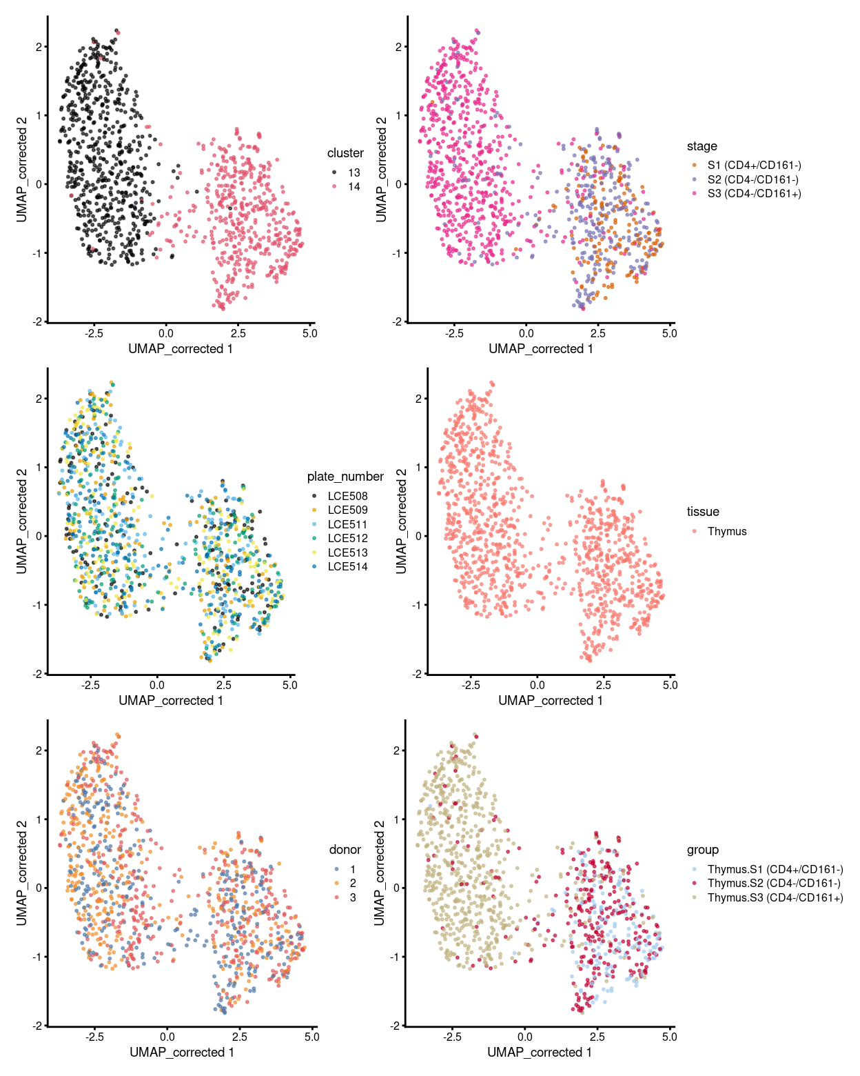
Figure 1: UMAP plot, where each point represents a cell and is coloured according to the legend.
Show code
# summary - stacked barplot
p1 <- ggcells(sce) +
  geom_bar(aes(x = cluster, fill = cluster)) +
  coord_flip() +
  ylab("Number of samples") +
  theme_cowplot(font_size = 8) +
  scale_fill_manual(values = cluster_colours) +
  geom_text(stat='count', aes(x = cluster, label=..count..), hjust=1.5, size=2)
p2 <- ggcells(sce) +
  geom_bar(
    aes(x = cluster, fill = stage),
    position = position_fill(reverse = TRUE)) +
  coord_flip() +
  ylab("Frequency") +
  scale_fill_manual(values = stage_colours) +
  theme_cowplot(font_size = 8)
p3 <- ggcells(sce) +
  geom_bar(
    aes(x = cluster, fill = plate_number),
    position = position_fill(reverse = TRUE)) +
  coord_flip() +
  ylab("Frequency") +
  scale_fill_manual(values = plate_number_colours) +
  theme_cowplot(font_size = 8)
p4 <- ggcells(sce) +
  geom_bar(
    aes(x = cluster, fill = tissue),
    position = position_fill(reverse = TRUE)) +
  coord_flip() +
  ylab("Frequency") +
  scale_fill_manual(values = tissue_colours) +
  theme_cowplot(font_size = 8)
p5 <- ggcells(sce) +
  geom_bar(
    aes(x = cluster, fill = donor),
    position = position_fill(reverse = TRUE)) +
  coord_flip() +
  ylab("Frequency") +
  scale_fill_manual(values = donor_colours) +
  theme_cowplot(font_size = 8)
p6 <- ggcells(sce) +
  geom_bar(
    aes(x = cluster, fill = group),
    position = position_fill(reverse = TRUE)) +
  coord_flip() +
  ylab("Frequency") +
  scale_fill_manual(values = group_colours) +
  theme_cowplot(font_size = 8)
(p1 | p2) / (p3 | p4) / (p5 | p6)
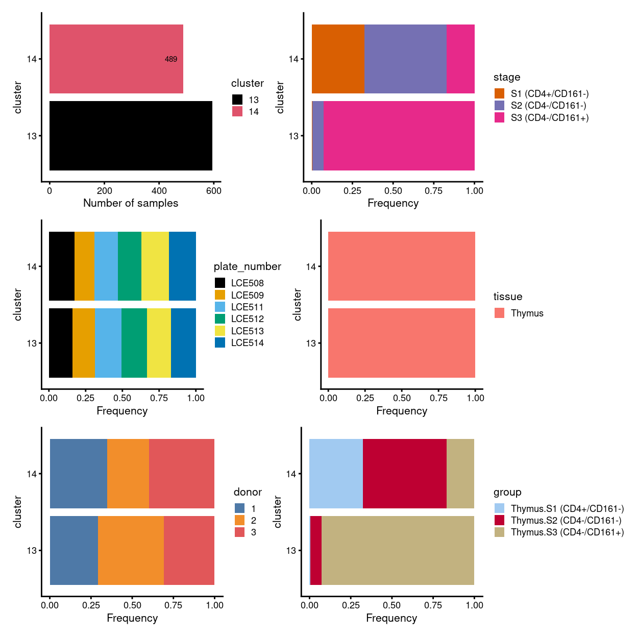
Figure 2: Breakdown of clusters by experimental factors.
NOTE: Considering the fact that SingleR with use of the annotation reference (Monaco Immune Cell Data) most relevant to the gamma-delta T cells (even annotated at cell level) could not further sub-classify the developmental stage/subtype of them (either annotating cluster as Th1 cell-/Naive CD8/CD4 T cell or Vd2gd T cells-alike) [ref: EDA_annotation_SingleR_MI_fine_cell_level.R], we decide to characterize the clusters by manual detection and curation of specific marker genes directly.
Marker gene detection
To interpret our clustering results, we identify the genes that drive separation between clusters. These marker genes allow us to assign biological meaning to each cluster based on their functional annotation. In the most obvious case, the marker genes for each cluster are a priori associated with particular cell types, allowing us to treat the clustering as a proxy for cell type identity. The same principle can be applied to more subtle differences in activation status or differentiation state.
Identification of marker genes is usually based around the retrospective detection of differential expression between clusters1. Genes that are more strongly DE are more likely to have driven cluster separation in the first place. The top DE genes are likely to be good candidate markers as they can effectively distinguish between cells in different clusters.
The Welch t-test is an obvious choice of statistical method to test for differences in expression between clusters. It is quickly computed and has good statistical properties for large numbers of cells (Soneson and Robinson 2018).
Show code
# block on plate
sce$block <- paste0(sce$plate_number)
Cluster 13 vs. 14
Here we look for the unique up-regulated markers of each cluster when compared to the all remaining ones.
Show code
###################################
# (M1) raw unique
#
# cluster 13 (i.e. mostly.thymus.S3.with.S1.S2)
# cluster 14 (i.e. mostly.thymus.S1.S2)

# find unique DE ./. clusters
uniquely_up <- findMarkers(
  sce,
  groups = sce$cluster,
  block = sce$block,
  pval.type = "all",
  direction = "up")
Show code
# export DGE lists
saveRDS(
  uniquely_up,
  here("data", "marker_genes", "thymus_only", "C094_Pellicci.uniquely_up.cluster_13_vs_14.rds"),
  compress = "xz")

dir.create(here("output", "marker_genes", "thymus_only", "uniquely_up", "cluster_13_vs_14"), recursive = TRUE)

vs_pair <- c("13", "14")

message("Writing 'uniquely_up (cluster_13_vs_14)' marker genes to file.")
for (n in names(uniquely_up)) {
  message(n)
  gzout <- gzfile(
    description = here(
      "output",
      "marker_genes",
      "thymus_only",
      "uniquely_up",
      "cluster_13_vs_14",
      paste0("cluster_",
             vs_pair[which(names(uniquely_up) %in% n)],
             "_vs_",
             vs_pair[-which(names(uniquely_up) %in% n)][1],
             "_vs_",
             vs_pair[-which(names(uniquely_up) %in% n)][2],
             ".uniquely_up.csv.gz")),
    open = "wb")
  write.table(
    x = uniquely_up[[n]] %>%
      as.data.frame() %>%
      tibble::rownames_to_column("gene_ID"),
    file = gzout,
    sep = ",",
    quote = FALSE,
    row.names = FALSE,
    col.names = TRUE)
  close(gzout)
}
Show code
# NOTE: The following is a workaround to the lack of support for tabsets in
#       distill (see https://github.com/rstudio/distill/issues/11 and
#       https://github.com/rstudio/distill/issues/11#issuecomment-692142414 in
#       particular).
xaringanExtra::use_panelset()
Cluster 13
Show code
##########################################
# look at cluster 13 (i.e. mostly.thymus.S3.with.S1.S2)
chosen <- "13"
cluster13_uniquely_up <- uniquely_up[[chosen]]

# add description for the chosen cluster-group
x <- "(mostly.thymus.S3.with.S1.S2)"

# look only at protein coding gene (pcg)
# NOTE: not suggest to narrow down into pcg as it remove all significant candidates (FDR << 0.05) !
# cluster13_uniquely_up <- cluster13_uniquely_up[intersect(protein_coding_gene_set, rownames(cluster13_uniquely_up)), ]

# get rid of noise (i.e. pseudo, ribo, mito, sex) that collaborator not interested in
cluster13_uniquely_up_noiseR <- cluster13_uniquely_up[setdiff(rownames(cluster13_uniquely_up), c(pseudogene_set, mito_set, ribo_set, sex_set)), ]

# see if key marker, "CD4 and/or ""KLRB1/CD161"", contain in the DE list + if it is "significant (i.e FDR <0.05)
y <- c("CD4",
       which(rownames(cluster13_uniquely_up_noiseR) %in% "CD4"),
       cluster13_uniquely_up_noiseR[which(rownames(cluster13_uniquely_up_noiseR) %in% "CD4"), ]$FDR < 0.05)
z <- c("KLRB1/CD161",
       which(rownames(cluster13_uniquely_up_noiseR) %in% "KLRB1"),
       cluster13_uniquely_up_noiseR[which(rownames(cluster13_uniquely_up_noiseR) %in% "KLRB1"), ]$FDR < 0.05)

# top25 only
best_set <- cluster13_uniquely_up_noiseR[1:25, ]
Show code
# heatmap
plotHeatmap(
  sce,
  features = rownames(best_set),
  columns = order(
    sce$cluster,
    sce$stage,
    sce$tissue,
    sce$donor,
    sce$group,
    sce$plate_number,
    sce$CD4,
    sce$CD161),
  colour_columns_by = c(
    "cluster",
    "stage",
    "tissue",
    "donor",
    "group",
    "plate_number",
    "CD4",
    "CD161"),
  cluster_cols = FALSE,
  center = TRUE,
  symmetric = TRUE,
  zlim = c(-3, 3),
  show_colnames = FALSE,
  annotation_row = data.frame(
    Sig = factor(
      ifelse(best_set[, "FDR"] < 0.05, "Yes", "No"),
      # TODO: temp trick to deal with the row-colouring problem
      # levels = c("Yes", "No")),
      levels = c("Yes")),
    row.names = rownames(best_set)),
  main = paste0("Cluster ", chosen, " ", x, " - \n",
                y[1], "_top ", y[2], "_significance: ", y[3], " ; \n",
                z[1], "_top ", z[2], "_significance: ", z[3]),
  column_annotation_colors = list(
    # Sig = c("Yes" = "red", "No" = "lightgrey"),
    cluster = cluster_colours,
    stage = stage_colours,
    tissue = tissue_colours,
    donor = donor_colours,
    group = group_colours,
    plate_number = plate_number_colours),
  color = hcl.colors(101, "Blue-Red 3"),
  fontsize = 7)
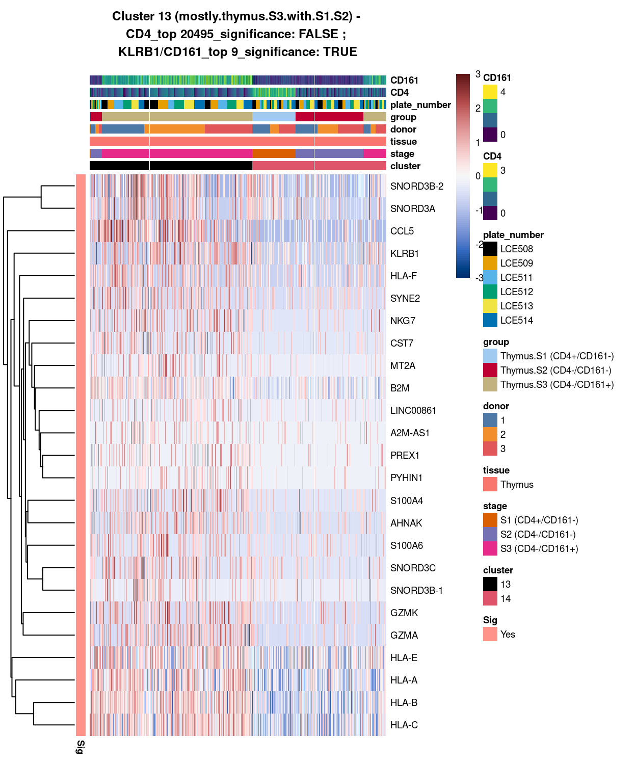
Figure 3: Heatmap of log-expression values in each sample for the top uniquely upregulated marker genes. Each column is a sample, each row a gene. Colours are capped at -3 and 3 to preserve dynamic range. Ranking of CD4 and CD161/KLRB1 from top of the DGE list sorted in ascending order of FDR and their statistical significance (TRUE = FDR < 0.05) are provided in the title
Cluster 14
Show code
##########################################
# look at cluster 14 (i.e. mostly.thymus.S1.S2)
chosen <- "14"
cluster14_uniquely_up <- uniquely_up[[chosen]]

# add description for the chosen cluster-group
x <- "(mostly.thymus.S1.S2)"

# look only at protein coding gene (pcg)
# NOTE: not suggest to narrow down into pcg as it remove all significant candidates (FDR << 0.05) !
# cluster14_uniquely_up <- cluster14_uniquely_up[intersect(protein_coding_gene_set, rownames(cluster14_uniquely_up)), ]

# get rid of noise (i.e. pseudo, ribo, mito, sex) that collaborator not interested in
cluster14_uniquely_up_noiseR <- cluster14_uniquely_up[setdiff(rownames(cluster14_uniquely_up), c(pseudogene_set, mito_set, ribo_set, sex_set)), ]

# see if key marker, "CD4 and/or ""KLRB1/CD161"", contain in the DE list + if it is "significant (i.e FDR <0.05)
y <- c("CD4",
       which(rownames(cluster14_uniquely_up_noiseR) %in% "CD4"),
       cluster14_uniquely_up_noiseR[which(rownames(cluster14_uniquely_up_noiseR) %in% "CD4"), ]$FDR < 0.05)
z <- c("KLRB1/CD161",
       which(rownames(cluster14_uniquely_up_noiseR) %in% "KLRB1"),
       cluster14_uniquely_up_noiseR[which(rownames(cluster14_uniquely_up_noiseR) %in% "KLRB1"), ]$FDR < 0.05)

# top25 only
best_set <- cluster14_uniquely_up_noiseR[1:25, ]
Show code
# heatmap
plotHeatmap(
  sce,
  features = rownames(best_set),
  columns = order(
    sce$cluster,
    sce$stage,
    sce$tissue,
    sce$donor,
    sce$group,
    sce$plate_number,
    sce$CD4,
    sce$CD161),
  colour_columns_by = c(
    "cluster",
    "stage",
    "tissue",
    "donor",
    "group",
    "plate_number",
    "CD4",
    "CD161"),
  cluster_cols = FALSE,
  center = TRUE,
  symmetric = TRUE,
  zlim = c(-3, 3),
  show_colnames = FALSE,
  annotation_row = data.frame(
    Sig = factor(
      ifelse(best_set[, "FDR"] < 0.05, "Yes", "No"),
      # TODO: temp trick to deal with the row-colouring problem
      # levels = c("Yes", "No")),
      levels = c("Yes")),
    row.names = rownames(best_set)),
  main = paste0("Cluster ", chosen, " ", x, " - \n",
                y[1], "_top ", y[2], "_significance: ", y[3], " ; \n",
                z[1], "_top ", z[2], "_significance: ", z[3]),
  column_annotation_colors = list(
    # Sig = c("Yes" = "red", "No" = "lightgrey"),
    cluster = cluster_colours,
    stage = stage_colours,
    tissue = tissue_colours,
    donor = donor_colours,
    group = group_colours,
    plate_number = plate_number_colours),
  color = hcl.colors(101, "Blue-Red 3"),
  fontsize = 7)
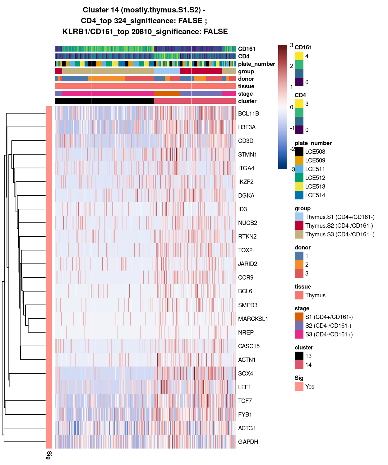
Figure 4: Heatmap of log-expression values in each sample for the top uniquely upregulated marker genes. Each column is a sample, each row a gene. Colours are capped at -3 and 3 to preserve dynamic range. Ranking of CD4 and CD161/KLRB1 from top of the DGE list sorted in ascending order of FDR and their statistical significance (TRUE = FDR < 0.05) are provided in the title
DGE lists of these comparisons are available in output/marker_genes/thymus_only/uniquely_up/cluster_13_vs_14/.
Summary:
For the thymus only subset, one would expect that there are at least 3 different groups of cells, ie. thymus.s1, thymus.s2, thymus.s3, upon clustering. But due to the high similarities between the thymus.S1 and thymus.S2 cells, where even in the mini-bulk setting, there are only 17 differentially expressed genes can be detected. Therefore, during the clustering of this subset of single cells, we may hope to separate the thymus.S1 and thymus.S2 cells. But unfortunately, increasing the number of clusters cannot achieve this purpose, but only further divide cells in the thymus.S3 cells into 2 to 3 subgroups.
For the thymus.S3 subgroups, we did try to test if cells contained in higher number of clusters are truly different, but based on the outcome of our statistical DE test, these sub-groups show no difference from each other and thus should be combined.
On the whole, the best we can achieve from the single-cell samples of the thymus only subset could be to compare the difference between the thymus.S1.S2-mix and the thymus.S3, then make use of it to perhaps validate the mini-bulk outcome.
Expression of minibulk DE in the single-cell dataset
Show code
###############################################
# Heatmap using minibulk sig markers as feature

# laod package for read in csv.gz
library(data.table)
library(R.utils)

# read in
a <- fread(here("output", "DEGs", "excluding_blood_1-3", "Thymus.S3_vs_Thymus.S1.aggregated_tech_reps.DEGs.csv.gz"))
b <- fread(here("output", "DEGs", "excluding_blood_1-3", "Thymus.S2_vs_Thymus.S1.aggregated_tech_reps.DEGs.csv.gz"))
c <- fread(here("output", "DEGs", "excluding_blood_1-3", "Thymus.S3_vs_Thymus.S2.aggregated_tech_reps.DEGs.csv.gz"))

# extract DEGlist (FDR < 0.05)
minibulkDEG.a <- a$ENSEMBL.GENENAME[a$FDR<0.05]
minibulkDEG.b <- b$ENSEMBL.GENENAME[b$FDR<0.05]
minibulkDEG.c <- c$ENSEMBL.GENENAME[c$FDR<0.05]

minibulkDEG.a.up <- a$ENSEMBL.GENENAME[a$FDR<0.05 & a$logFC>0]
minibulkDEG.b.up <- b$ENSEMBL.GENENAME[b$FDR<0.05 & b$logFC>0]
minibulkDEG.c.up <- c$ENSEMBL.GENENAME[c$FDR<0.05 & c$logFC>0]

minibulkDEG.a.down <- a$ENSEMBL.GENENAME[a$FDR<0.05 & a$logFC<0]
minibulkDEG.b.down <- b$ENSEMBL.GENENAME[b$FDR<0.05 & b$logFC<0]
minibulkDEG.c.down <- c$ENSEMBL.GENENAME[c$FDR<0.05 & c$logFC<0]

# keep only unique markers
uniq.minibulkDEG.a <- Reduce(setdiff, list(minibulkDEG.a,
                                           minibulkDEG.b,
                                           minibulkDEG.c))
uniq.minibulkDEG.b <- Reduce(setdiff, list(minibulkDEG.b,
                                           minibulkDEG.a,
                                           minibulkDEG.c))
uniq.minibulkDEG.c <- Reduce(setdiff, list(minibulkDEG.c,
                                           minibulkDEG.a,
                                           minibulkDEG.b))

uniq.minibulkDEG.a.up <- Reduce(setdiff, list(minibulkDEG.a.up,
                                              minibulkDEG.b.up,
                                              minibulkDEG.c.up))
uniq.minibulkDEG.b.up <- Reduce(setdiff, list(minibulkDEG.b.up,
                                              minibulkDEG.a.up,
                                              minibulkDEG.c.up))
uniq.minibulkDEG.c.up <- Reduce(setdiff, list(minibulkDEG.c.up,
                                              minibulkDEG.a.up,
                                              minibulkDEG.b.up))

uniq.minibulkDEG.a.down <- Reduce(setdiff, list(minibulkDEG.a.down,
                                                minibulkDEG.b.down,
                                                minibulkDEG.c.down))
uniq.minibulkDEG.b.down <- Reduce(setdiff, list(minibulkDEG.b.down,
                                                minibulkDEG.a.down,
                                                minibulkDEG.c.down))
uniq.minibulkDEG.c.down <- Reduce(setdiff, list(minibulkDEG.c.down,
                                                minibulkDEG.a.down,
                                                minibulkDEG.b.down))

# check number of unique minibulkDEG in each
length(uniq.minibulkDEG.a)
[1] 514Show code
length(uniq.minibulkDEG.b)
[1] 3Show code
length(uniq.minibulkDEG.c)
[1] 40Show code
length(uniq.minibulkDEG.a.up)
[1] 223Show code
length(uniq.minibulkDEG.b.up)
[1] 2Show code
length(uniq.minibulkDEG.c.up)
[1] 18Show code
length(uniq.minibulkDEG.a.down)
[1] 291Show code
length(uniq.minibulkDEG.b.down)
[1] 2Show code
length(uniq.minibulkDEG.c.down)
[1] 23Show code
# keep only top25
top.uniq.minibulkDEG.a <- if(length(uniq.minibulkDEG.a) >=25){uniq.minibulkDEG.a[1:25]} else {uniq.minibulkDEG.a}
top.uniq.minibulkDEG.b <- if(length(uniq.minibulkDEG.b) >=25){uniq.minibulkDEG.b[1:25]} else {uniq.minibulkDEG.b}
top.uniq.minibulkDEG.c <- if(length(uniq.minibulkDEG.c) >=25){uniq.minibulkDEG.c[1:25]} else {uniq.minibulkDEG.c}

top.uniq.minibulkDEG.a.up <- if(length(uniq.minibulkDEG.a.up) >=25){uniq.minibulkDEG.a.up[1:25]} else {uniq.minibulkDEG.a.up}
top.uniq.minibulkDEG.b.up <- if(length(uniq.minibulkDEG.b.up) >=25){uniq.minibulkDEG.b.up[1:25]} else {uniq.minibulkDEG.b.up}
top.uniq.minibulkDEG.c.up <- if(length(uniq.minibulkDEG.c.up) >=25){uniq.minibulkDEG.c.up[1:25]} else {uniq.minibulkDEG.c.up}

top.uniq.minibulkDEG.a.down <- if(length(uniq.minibulkDEG.a.down) >=25){uniq.minibulkDEG.a.down[1:25]} else {uniq.minibulkDEG.a.down}
top.uniq.minibulkDEG.b.down <- if(length(uniq.minibulkDEG.b.down) >=25){uniq.minibulkDEG.b.down[1:25]} else {uniq.minibulkDEG.b.down}
top.uniq.minibulkDEG.c.down <- if(length(uniq.minibulkDEG.c.down) >=25){uniq.minibulkDEG.c.down[1:25]} else {uniq.minibulkDEG.c.down}

# feature
minibulk_markers <- c(top.uniq.minibulkDEG.a,
                      top.uniq.minibulkDEG.b,
                      top.uniq.minibulkDEG.c)

minibulk_markers_up <- c(top.uniq.minibulkDEG.a.up,
                         top.uniq.minibulkDEG.b.up,
                         top.uniq.minibulkDEG.c.up)

minibulk_markers_down <- c(top.uniq.minibulkDEG.a.down,
                           top.uniq.minibulkDEG.b.down,
                           top.uniq.minibulkDEG.c.down)
Show code
# NOTE: The following is a workaround to the lack of support for tabsets in
#       distill (see https://github.com/rstudio/distill/issues/11 and
#       https://github.com/rstudio/distill/issues/11#issuecomment-692142414 in
#       particular).
xaringanExtra::use_panelset()
Minibulk DE_ALL_by cluster
Show code
library(scater)
plotHeatmap(
  sce,
  features = minibulk_markers,
  columns = order(
    sce$cluster,
    sce$stage,
    sce$tissue,
    sce$donor,
    sce$group,
    sce$plate_number),
  colour_columns_by = c(
    "cluster",
    "stage",
    "tissue",
    "donor",
    "group",
    "plate_number"),
  cluster_cols = FALSE,
  center = TRUE,
  symmetric = TRUE,
  zlim = c(-3, 3),
  show_colnames = FALSE,
  # TODO: temp trick to deal with the row-colouring problem
  annotation_row = data.frame(
    thymus.s3.vs.thymus.s1 = factor(ifelse(minibulk_markers %in% top.uniq.minibulkDEG.a, "DE", "not DE"), levels = c("DE")),
    thymus.s2.vs.thymus.s1 = factor(ifelse(minibulk_markers %in% top.uniq.minibulkDEG.b, "DE", "not DE"), levels = c("DE")),
    thymus.s3.vs.thymus.s2 = factor(ifelse(minibulk_markers %in% top.uniq.minibulkDEG.c, "DE", "not DE"), levels = c("DE")),
    row.names = minibulk_markers),
  main = "Minibulk DE expression (UP and DOWN) in thymus subset (with cells divided by clusters)",
  column_annotation_colors = list(
    cluster = cluster_colours,
    stage = stage_colours,
    tissue = tissue_colours,
    donor = donor_colours,
    group = group_colours,
    plate_number = plate_number_colours),
  color = hcl.colors(101, "Blue-Red 3"),
  fontsize = 7)
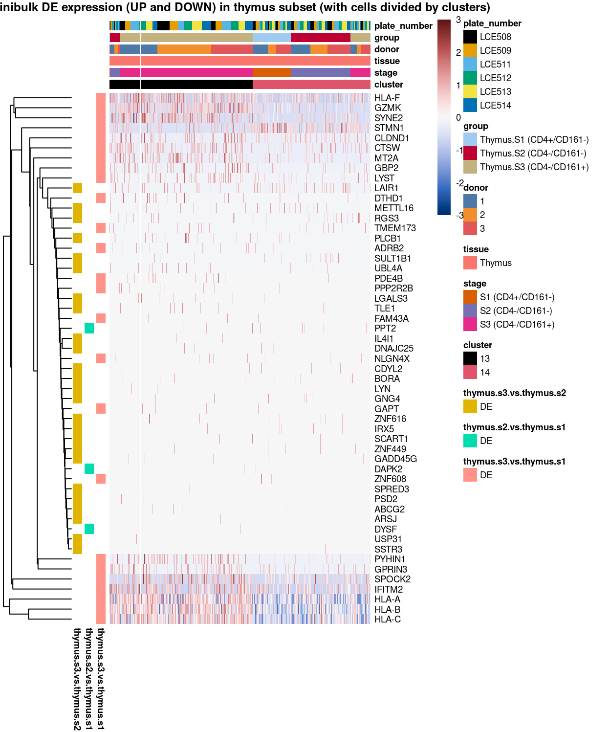
Figure 5: Heatmap of log-expression values in each sample for the marker genes identified from the mini-bulk analysis. Cells are ordered by cluster. Each column is a sample, each row a gene. Colours are capped at -3 and 3 to preserve dynamic range.
Minibulk DE_ALL_by group
Show code
library(scater)
plotHeatmap(
  sce,
  features = minibulk_markers,
  columns = order(
    sce$group,
    sce$stage,
    sce$tissue,
    sce$donor,
    sce$plate_number),
  colour_columns_by = c(
    "group",
    "stage",
    "tissue",
    "donor",
    "plate_number"),
  cluster_cols = FALSE,
  center = TRUE,
  symmetric = TRUE,
  zlim = c(-3, 3),
  show_colnames = FALSE,
  # TODO: temp trick to deal with the row-colouring problem
  annotation_row = data.frame(
    thymus.s3.vs.thymus.s1 = factor(ifelse(minibulk_markers %in% top.uniq.minibulkDEG.a, "DE", "not DE"), levels = c("DE")),
    thymus.s2.vs.thymus.s1 = factor(ifelse(minibulk_markers %in% top.uniq.minibulkDEG.b, "DE", "not DE"), levels = c("DE")),
    thymus.s3.vs.thymus.s2 = factor(ifelse(minibulk_markers %in% top.uniq.minibulkDEG.c, "DE", "not DE"), levels = c("DE")),
    row.names = minibulk_markers),
  main = "Minibulk DE expression (UP and DOWN) in thymus subset (with cells divided by groups)",
  column_annotation_colors = list(
    group = group_colours,
    stage = stage_colours,
    tissue = tissue_colours,
    donor = donor_colours,
    plate_number = plate_number_colours),
  color = hcl.colors(101, "Blue-Red 3"),
  fontsize = 7)
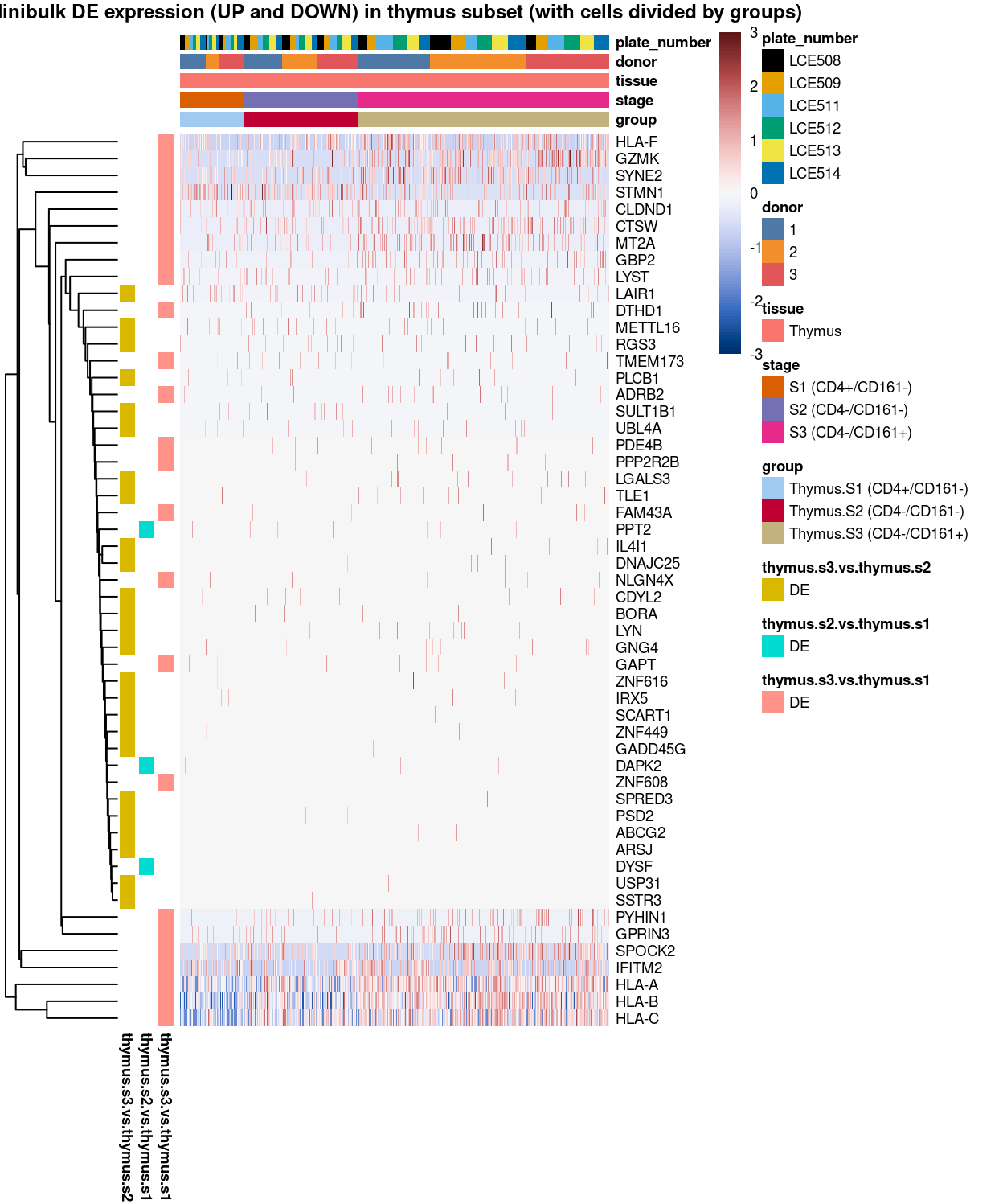
Figure 6: Heatmap of log-expression values in each sample for the marker genes identified from the mini-bulk analysis. Cells are ordered by group. Each column is a sample, each row a gene. Colours are capped at -3 and 3 to preserve dynamic range.
Minibulk DE_ALL_by group (clust_col)
Show code
library(scater)
plotHeatmap(
  sce,
  features = minibulk_markers,
  columns = order(
    sce$group,
    sce$stage,
    sce$tissue,
    sce$donor,
    sce$plate_number),
  colour_columns_by = c(
    "group",
    "stage",
    "tissue",
    "donor",
    "plate_number"),
  cluster_cols = TRUE,
  center = TRUE,
  symmetric = TRUE,
  zlim = c(-3, 3),
  show_colnames = FALSE,
  # TODO: temp trick to deal with the row-colouring problem
  annotation_row = data.frame(
    thymus.s3.vs.thymus.s1 = factor(ifelse(minibulk_markers %in% top.uniq.minibulkDEG.a, "DE", "not DE"), levels = c("DE")),
    thymus.s2.vs.thymus.s1 = factor(ifelse(minibulk_markers %in% top.uniq.minibulkDEG.b, "DE", "not DE"), levels = c("DE")),
    thymus.s3.vs.thymus.s2 = factor(ifelse(minibulk_markers %in% top.uniq.minibulkDEG.c, "DE", "not DE"), levels = c("DE")),
    row.names = minibulk_markers),
  main = "Minibulk DE expression (UP and DOWN) in thymus subset (with cells divided by groups, column-clustered)",
  column_annotation_colors = list(
    group = group_colours,
    stage = stage_colours,
    tissue = tissue_colours,
    donor = donor_colours,
    plate_number = plate_number_colours),
  color = hcl.colors(101, "Blue-Red 3"),
  fontsize = 7)
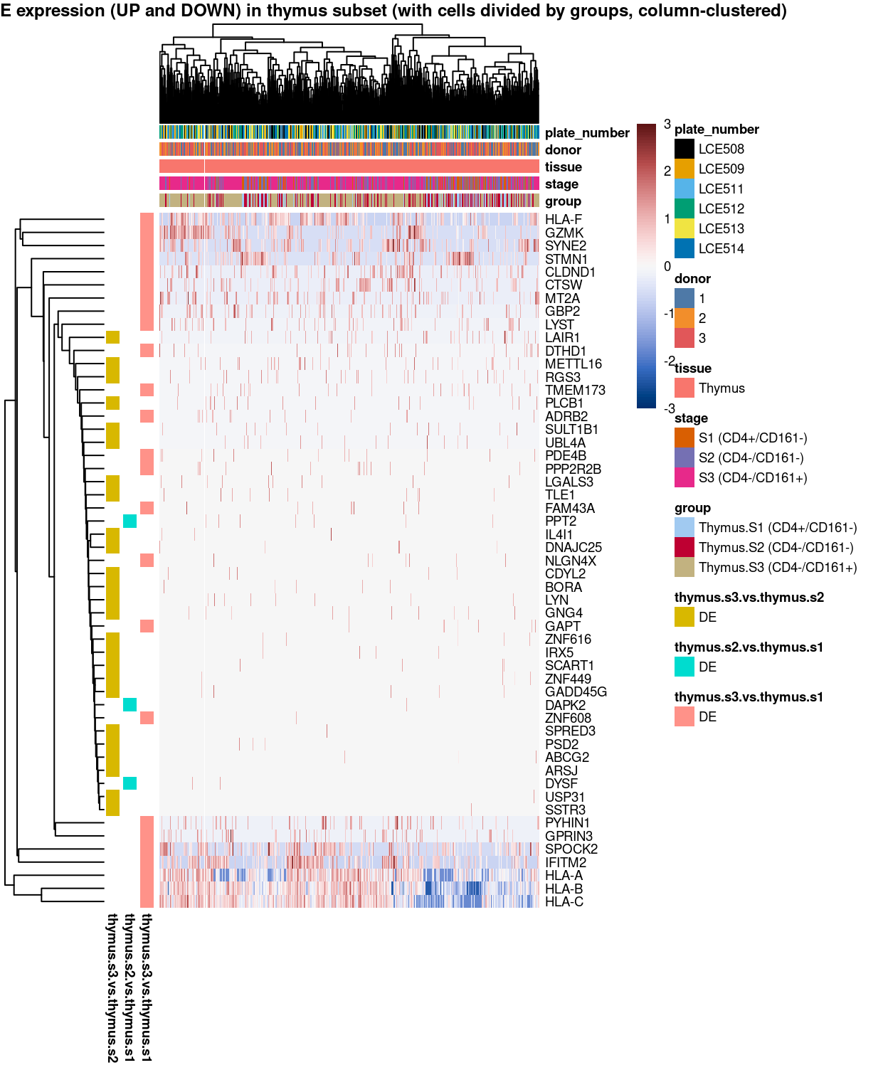
Figure 7: Heatmap of log-expression values in each sample for the marker genes identified from the mini-bulk analysis. Cells are ordered by group (column-clustered). Each column is a sample, each row a gene. Colours are capped at -3 and 3 to preserve dynamic range.
Minibulk DE_UP_by cluster
Show code
library(scater)
plotHeatmap(
  sce,
  features = minibulk_markers_up,
  columns = order(
    sce$cluster,
    sce$stage,
    sce$tissue,
    sce$donor,
    sce$group,
    sce$plate_number),
  colour_columns_by = c(
    "cluster",
    "stage",
    "tissue",
    "donor",
    "group",
    "plate_number"),
  cluster_cols = FALSE,
  center = TRUE,
  symmetric = TRUE,
  zlim = c(-3, 3),
  show_colnames = FALSE,
  # TODO: temp trick to deal with the row-colouring problem
  annotation_row = data.frame(
    thymus.s3.vs.thymus.s1 = factor(ifelse(minibulk_markers_up %in% top.uniq.minibulkDEG.a.up, "DE", "not DE"), levels = c("DE")),
    thymus.s2.vs.thymus.s1 = factor(ifelse(minibulk_markers_up %in% top.uniq.minibulkDEG.b.up, "DE", "not DE"), levels = c("DE")),
    thymus.s3.vs.thymus.s2 = factor(ifelse(minibulk_markers_up %in% top.uniq.minibulkDEG.c.up, "DE", "not DE"), levels = c("DE")),
    row.names = minibulk_markers_up),
  main = "Minibulk DE expression (UP only) in thymus subset (with cells divided by clusters)",
  column_annotation_colors = list(
    cluster = cluster_colours,
    stage = stage_colours,
    tissue = tissue_colours,
    donor = donor_colours,
    group = group_colours,
    plate_number = plate_number_colours),
  color = hcl.colors(101, "Blue-Red 3"),
  fontsize = 7)
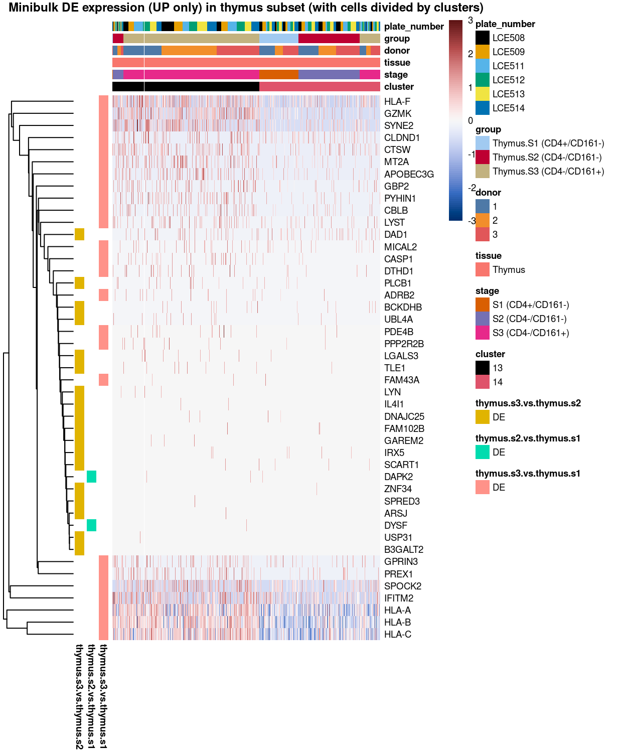
Figure 8: Heatmap of log-expression values in each sample for the marker genes (up-regulated) identified from the mini-bulk analysis. Cells are ordered by cluster. Each column is a sample, each row a gene. Colours are capped at -3 and 3 to preserve dynamic range.
Minibulk DE_UP_by group
Show code
library(scater)
plotHeatmap(
  sce,
  features = minibulk_markers_up,
  columns = order(
    sce$group,
    sce$stage,
    sce$tissue,
    sce$donor,
    sce$plate_number),
  colour_columns_by = c(
    "group",
    "stage",
    "tissue",
    "donor",
    "plate_number"),
  cluster_cols = FALSE,
  center = TRUE,
  symmetric = TRUE,
  zlim = c(-3, 3),
  show_colnames = FALSE,
  # TODO: temp trick to deal with the row-colouring problem
  annotation_row = data.frame(
    thymus.s3.vs.thymus.s1 = factor(ifelse(minibulk_markers_up %in% top.uniq.minibulkDEG.a.up, "DE", "not DE"), levels = c("DE")),
    thymus.s2.vs.thymus.s1 = factor(ifelse(minibulk_markers_up %in% top.uniq.minibulkDEG.b.up, "DE", "not DE"), levels = c("DE")),
    thymus.s3.vs.thymus.s2 = factor(ifelse(minibulk_markers_up %in% top.uniq.minibulkDEG.c.up, "DE", "not DE"), levels = c("DE")),
    row.names = minibulk_markers_up),
  main = "Minibulk DE expression (UP only) in thymus subset (with cells divided by groups)",
  column_annotation_colors = list(
    group = group_colours,
    stage = stage_colours,
    tissue = tissue_colours,
    donor = donor_colours,
    plate_number = plate_number_colours),
  color = hcl.colors(101, "Blue-Red 3"),
  fontsize = 7)
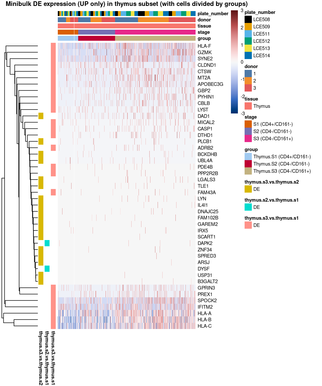
Figure 9: Heatmap of log-expression values in each sample for the marker genes (up-regulated) identified from the mini-bulk analysis. Cells are ordered by group. Each column is a sample, each row a gene. Colours are capped at -3 and 3 to preserve dynamic range.
Minibulk DE_UP_by group (clust_col)
Show code
library(scater)
plotHeatmap(
  sce,
  features = minibulk_markers_up,
  columns = order(
    sce$group,
    sce$stage,
    sce$tissue,
    sce$donor,
    sce$plate_number),
  colour_columns_by = c(
    "group",
    "stage",
    "tissue",
    "donor",
    "plate_number"),
  cluster_cols = TRUE,
  center = TRUE,
  symmetric = TRUE,
  zlim = c(-3, 3),
  show_colnames = FALSE,
  # TODO: temp trick to deal with the row-colouring problem
  annotation_row = data.frame(
    thymus.s3.vs.thymus.s1 = factor(ifelse(minibulk_markers_up %in% top.uniq.minibulkDEG.a.up, "DE", "not DE"), levels = c("DE")),
    thymus.s2.vs.thymus.s1 = factor(ifelse(minibulk_markers_up %in% top.uniq.minibulkDEG.b.up, "DE", "not DE"), levels = c("DE")),
    thymus.s3.vs.thymus.s2 = factor(ifelse(minibulk_markers_up %in% top.uniq.minibulkDEG.c.up, "DE", "not DE"), levels = c("DE")),
    row.names = minibulk_markers_up),
  main = "Minibulk DE expression (UP only) in thymus subset (with cells divided by groups, column-clustered)",
  column_annotation_colors = list(
    group = group_colours,
    stage = stage_colours,
    tissue = tissue_colours,
    donor = donor_colours,
    plate_number = plate_number_colours),
  color = hcl.colors(101, "Blue-Red 3"),
  fontsize = 7)
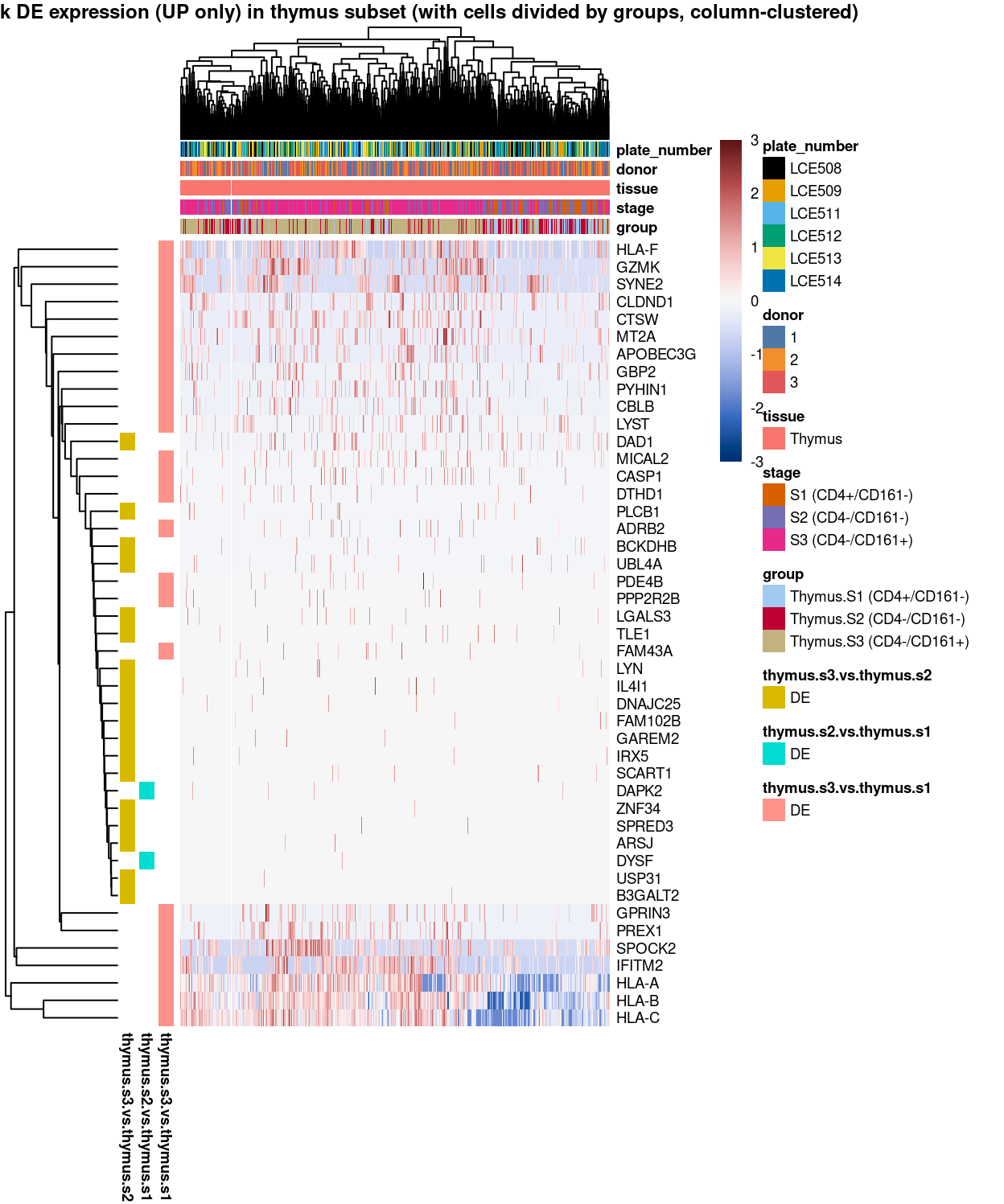
Figure 10: Heatmap of log-expression values in each sample for the marker genes (up-regulated) identified from the mini-bulk analysis. Cells are ordered by group (column-clustered). Each column is a sample, each row a gene. Colours are capped at -3 and 3 to preserve dynamic range.
Minibulk DE_DOWN_by cluster
Show code
library(scater)
plotHeatmap(
  sce,
  features = minibulk_markers_down,
  columns = order(
    sce$cluster,
    sce$stage,
    sce$tissue,
    sce$donor,
    sce$group,
    sce$plate_number),
  colour_columns_by = c(
    "cluster",
    "stage",
    "tissue",
    "donor",
    "group",
    "plate_number"),
  cluster_cols = FALSE,
  center = TRUE,
  symmetric = TRUE,
  zlim = c(-3, 3),
  show_colnames = FALSE,
  # TODO: temp trick to deal with the row-colouring problem
  annotation_row = data.frame(
    thymus.s3.vs.thymus.s1 = factor(ifelse(minibulk_markers_down %in% top.uniq.minibulkDEG.a.down, "DE", "not DE"), levels = c("DE")),
    thymus.s2.vs.thymus.s1 = factor(ifelse(minibulk_markers_down %in% top.uniq.minibulkDEG.b.down, "DE", "not DE"), levels = c("DE")),
    thymus.s3.vs.thymus.s2 = factor(ifelse(minibulk_markers_down %in% top.uniq.minibulkDEG.c.down, "DE", "not DE"), levels = c("DE")),
    row.names = minibulk_markers_down),
  main = "Minibulk DE expression (DOWN only) in thymus subset (with cells divided by clusters)",
  column_annotation_colors = list(
    cluster = cluster_colours,
    stage = stage_colours,
    tissue = tissue_colours,
    donor = donor_colours,
    group = group_colours,
    plate_number = plate_number_colours),
  color = hcl.colors(101, "Blue-Red 3"),
  fontsize = 7)
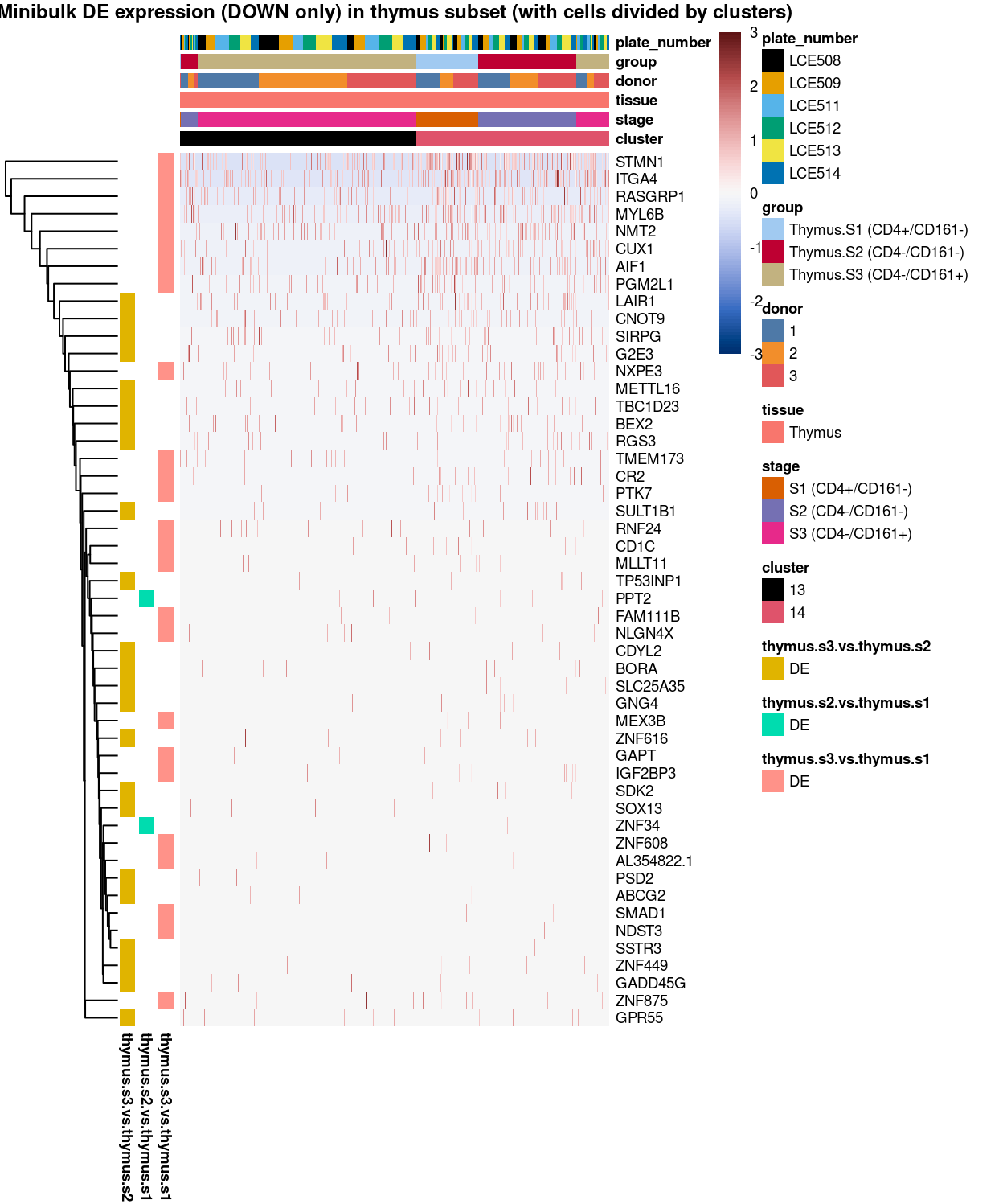
Figure 11: Heatmap of log-expression values in each sample for the marker genes (down-regulated) identified from the mini-bulk analysis. Cells are ordered by cluster. Each column is a sample, each row a gene. Colours are capped at -3 and 3 to preserve dynamic range.
Minibulk DE_DOWN_by group
Show code
library(scater)
plotHeatmap(
  sce,
  features = minibulk_markers_down,
  columns = order(
    sce$group,
    sce$stage,
    sce$tissue,
    sce$donor,
    sce$plate_number),
  colour_columns_by = c(
    "group",
    "stage",
    "tissue",
    "donor",
    "plate_number"),
  cluster_cols = FALSE,
  center = TRUE,
  symmetric = TRUE,
  zlim = c(-3, 3),
  show_colnames = FALSE,
  # TODO: temp trick to deal with the row-colouring problem
  annotation_row = data.frame(
    thymus.s3.vs.thymus.s1 = factor(ifelse(minibulk_markers_down %in% top.uniq.minibulkDEG.a.down, "DE", "not DE"), levels = c("DE")),
    thymus.s2.vs.thymus.s1 = factor(ifelse(minibulk_markers_down %in% top.uniq.minibulkDEG.b.down, "DE", "not DE"), levels = c("DE")),
    thymus.s3.vs.thymus.s2 = factor(ifelse(minibulk_markers_down %in% top.uniq.minibulkDEG.c.down, "DE", "not DE"), levels = c("DE")),
    row.names = minibulk_markers_down),
  main = "Minibulk DE expression (DOWN only) in thymus subset (with cells divided by groups)",
  column_annotation_colors = list(
    group = group_colours,
    stage = stage_colours,
    tissue = tissue_colours,
    donor = donor_colours,
    plate_number = plate_number_colours),
  color = hcl.colors(101, "Blue-Red 3"),
  fontsize = 7)
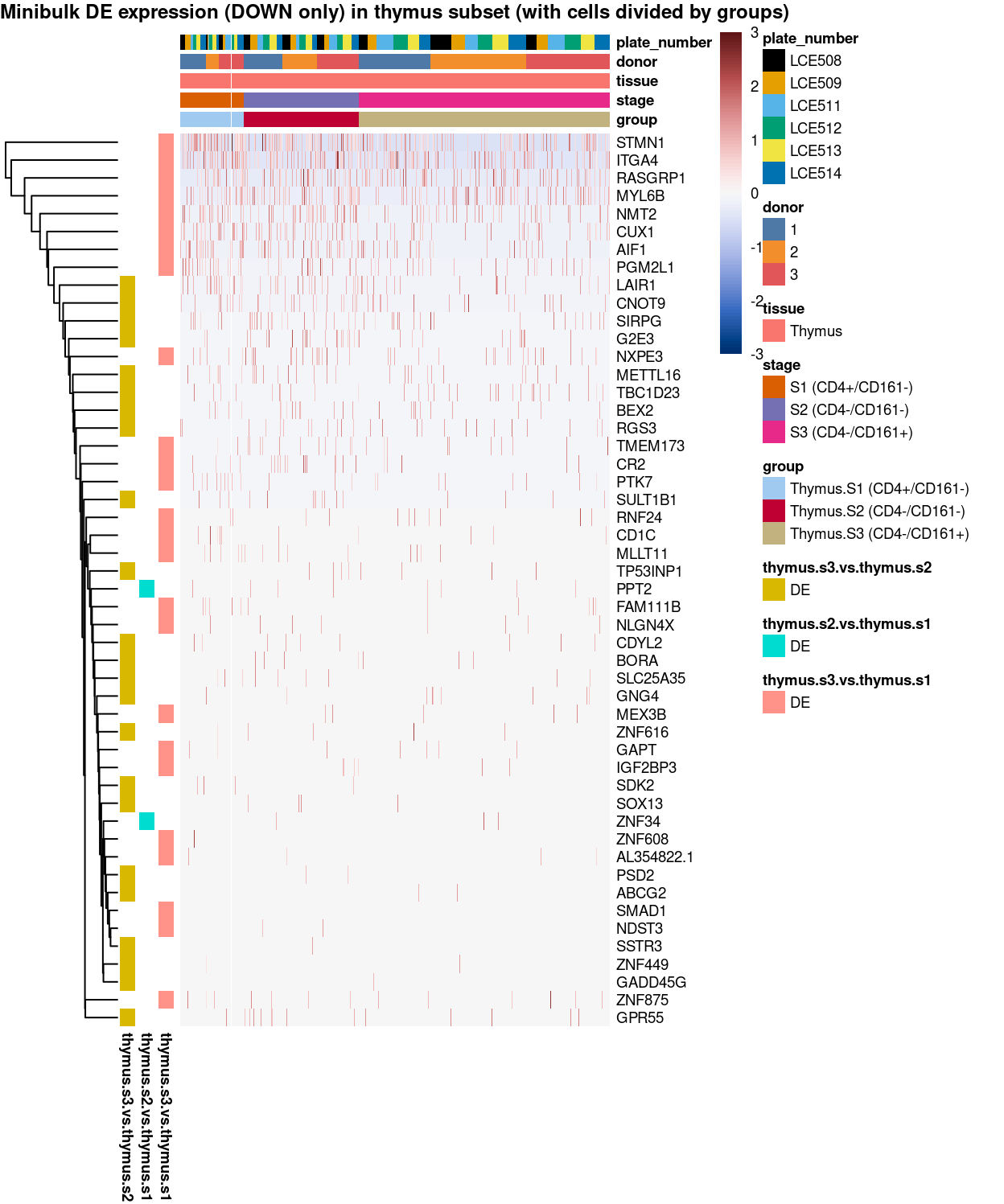
Figure 12: Heatmap of log-expression values in each sample for the marker genes (down-regulated) identified from the mini-bulk analysis. Cells are ordered by group. Each column is a sample, each row a gene. Colours are capped at -3 and 3 to preserve dynamic range.
Minibulk DE_DOWN_by group (clust_col)
Show code
library(scater)
plotHeatmap(
  sce,
  features = minibulk_markers_down,
  columns = order(
    sce$group,
    sce$stage,
    sce$tissue,
    sce$donor,
    sce$plate_number),
  colour_columns_by = c(
    "group",
    "stage",
    "tissue",
    "donor",
    "plate_number"),
  cluster_cols = TRUE,
  center = TRUE,
  symmetric = TRUE,
  zlim = c(-3, 3),
  show_colnames = FALSE,
  # TODO: temp trick to deal with the row-colouring problem
  annotation_row = data.frame(
    thymus.s3.vs.thymus.s1 = factor(ifelse(minibulk_markers_down %in% top.uniq.minibulkDEG.a.down, "DE", "not DE"), levels = c("DE")),
    thymus.s2.vs.thymus.s1 = factor(ifelse(minibulk_markers_down %in% top.uniq.minibulkDEG.b.down, "DE", "not DE"), levels = c("DE")),
    thymus.s3.vs.thymus.s2 = factor(ifelse(minibulk_markers_down %in% top.uniq.minibulkDEG.c.down, "DE", "not DE"), levels = c("DE")),
    row.names = minibulk_markers_down),
  main = "Minibulk DE expression (DOWN only) in thymus subset (with cells divided by groups, column-clustered)",
  column_annotation_colors = list(
    group = group_colours,
    stage = stage_colours,
    tissue = tissue_colours,
    donor = donor_colours,
    plate_number = plate_number_colours),
  color = hcl.colors(101, "Blue-Red 3"),
  fontsize = 7)
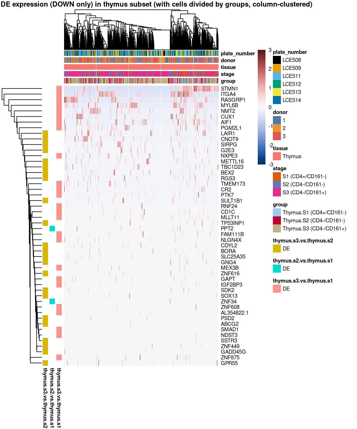
Figure 13: Heatmap of log-expression values in each sample for the marker genes (down-regulated) identified from the mini-bulk analysis. Cells are ordered by group (column-clustered). Each column is a sample, each row a gene. Colours are capped at -3 and 3 to preserve dynamic range.
Minibulk DE_ALL_by group (thymus.s3.vs.thymus.s1)
Show code
library(scater)
plotHeatmap(
  sce,
  features = top.uniq.minibulkDEG.a,
  columns = order(
    sce$group,
    sce$stage,
    sce$tissue,
    sce$donor,
    sce$plate_number),
  colour_columns_by = c(
    "group",
    "stage",
    "tissue",
    "donor",
    "plate_number"),
  cluster_cols = FALSE,
  center = TRUE,
  symmetric = TRUE,
  zlim = c(-3, 3),
  show_colnames = FALSE,
  # TODO: temp trick to deal with the row-colouring problem
  annotation_row = data.frame(
    thymus.s3.vs.thymus.s1 = factor(ifelse(minibulk_markers %in% top.uniq.minibulkDEG.a, "DE", "not DE"), levels = c("DE")),
    # thymus.s2.vs.thymus.s1 = factor(ifelse(minibulk_markers %in% top.uniq.minibulkDEG.b, "DE", "not DE"), levels = c("DE")),
    # thymus.s3.vs.thymus.s2 = factor(ifelse(minibulk_markers %in% top.uniq.minibulkDEG.c, "DE", "not DE"), levels = c("DE")),
    row.names = minibulk_markers),
  main = "Minibulk DE expression (thymus.S3 vs thymus.S1) in thymus subset (with cells divided by groups)",
  column_annotation_colors = list(
    group = group_colours,
    stage = stage_colours,
    tissue = tissue_colours,
    donor = donor_colours,
    plate_number = plate_number_colours),
  color = hcl.colors(101, "Blue-Red 3"),
  fontsize = 7)
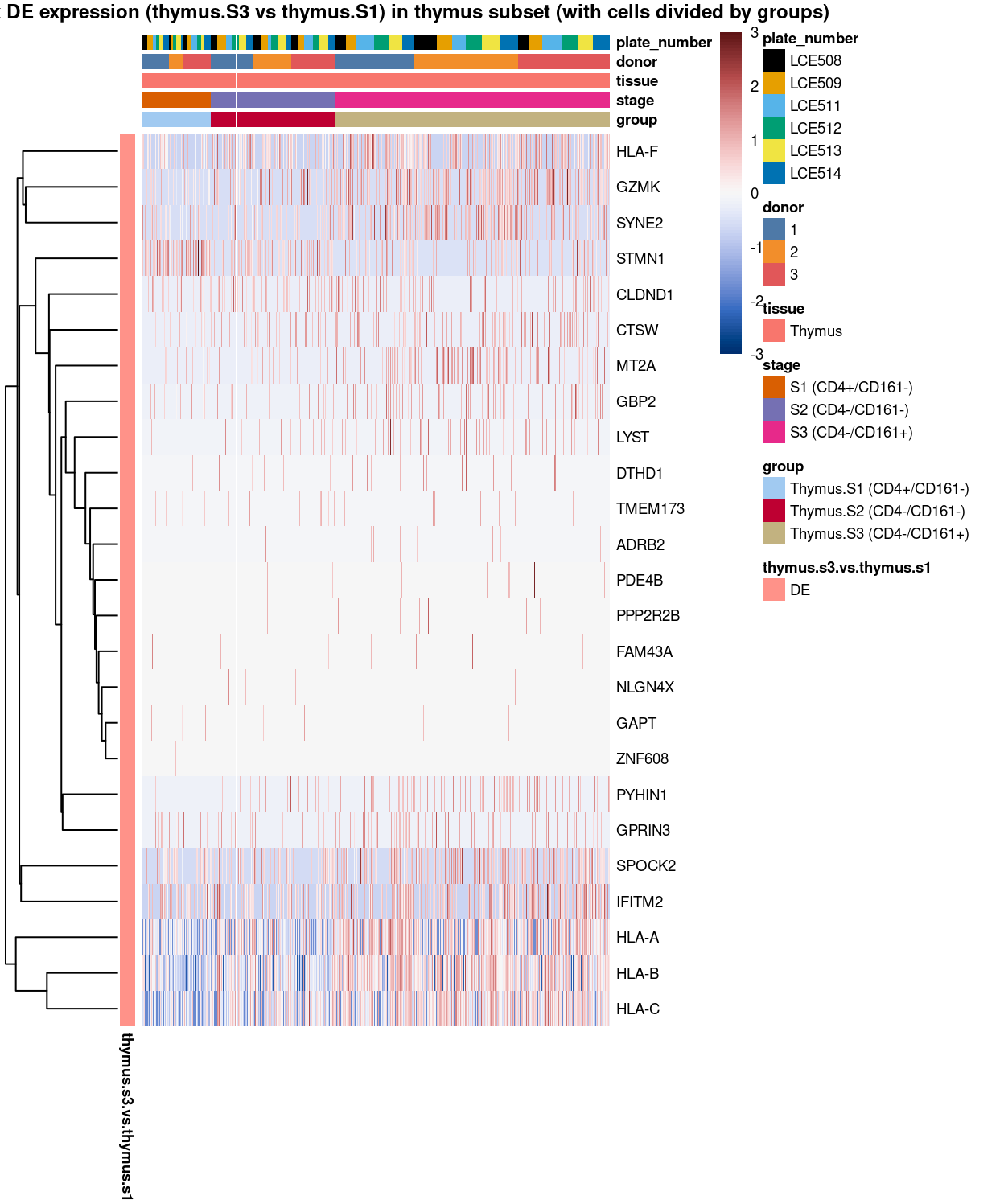
Figure 14: Heatmap of log-expression values in each sample for the marker genes identified from the mini-bulk analysis (thymus.s3.vs.thymus.s1). Cells are ordered by group. Each column is a sample, each row a gene. Colours are capped at -3 and 3 to preserve dynamic range.
Minibulk DE_ALL_by group (thymus.s2.vs.thymus.s1)
Show code
library(scater)
plotHeatmap(
  sce,
  features = top.uniq.minibulkDEG.b,
  columns = order(
    sce$group,
    sce$stage,
    sce$tissue,
    sce$donor,
    sce$plate_number),
  colour_columns_by = c(
    "group",
    "stage",
    "tissue",
    "donor",
    "plate_number"),
  cluster_cols = FALSE,
  center = TRUE,
  symmetric = TRUE,
  zlim = c(-3, 3),
  show_colnames = FALSE,
  # TODO: temp trick to deal with the row-colouring problem
  annotation_row = data.frame(
    # thymus.s3.vs.thymus.s1 = factor(ifelse(minibulk_markers %in% top.uniq.minibulkDEG.a, "DE", "not DE"), levels = c("DE")),
    thymus.s2.vs.thymus.s1 = factor(ifelse(minibulk_markers %in% top.uniq.minibulkDEG.b, "DE", "not DE"), levels = c("DE")),
    # thymus.s3.vs.thymus.s2 = factor(ifelse(minibulk_markers %in% top.uniq.minibulkDEG.c, "DE", "not DE"), levels = c("DE")),
    row.names = minibulk_markers),
  main = "Minibulk DE expression (thymus.S2 vs thymus.S1) in thymus subset (with cells divided by groups)",
  column_annotation_colors = list(
    group = group_colours,
    stage = stage_colours,
    tissue = tissue_colours,
    donor = donor_colours,
    plate_number = plate_number_colours),
  color = hcl.colors(101, "Blue-Red 3"),
  fontsize = 7)
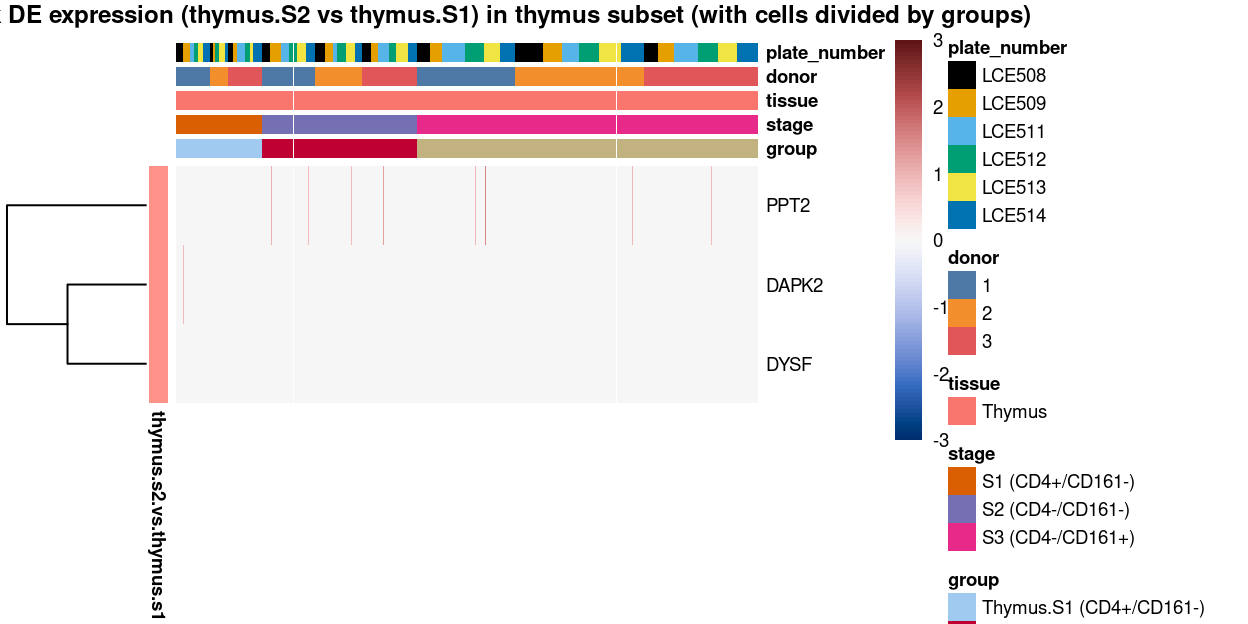
Figure 15: Heatmap of log-expression values in each sample for the marker genes identified from the mini-bulk analysis (thymus.s2.vs.thymus.s1). Cells are ordered by group. Each column is a sample, each row a gene. Colours are capped at -3 and 3 to preserve dynamic range.
Minibulk DE_ALL_by group (thymus.s3.vs.thymus.s2)
Show code
library(scater)
plotHeatmap(
  sce,
  features = top.uniq.minibulkDEG.c,
  columns = order(
    sce$group,
    sce$stage,
    sce$tissue,
    sce$donor,
    sce$plate_number),
  colour_columns_by = c(
    "group",
    "stage",
    "tissue",
    "donor",
    "plate_number"),
  cluster_cols = FALSE,
  center = TRUE,
  symmetric = TRUE,
  zlim = c(-3, 3),
  show_colnames = FALSE,
  # TODO: temp trick to deal with the row-colouring problem
  annotation_row = data.frame(
    # thymus.s3.vs.thymus.s1 = factor(ifelse(minibulk_markers %in% top.uniq.minibulkDEG.a, "DE", "not DE"), levels = c("DE")),
    # thymus.s2.vs.thymus.s1 = factor(ifelse(minibulk_markers %in% top.uniq.minibulkDEG.b, "DE", "not DE"), levels = c("DE")),
    thymus.s3.vs.thymus.s2 = factor(ifelse(minibulk_markers %in% top.uniq.minibulkDEG.c, "DE", "not DE"), levels = c("DE")),
    row.names = minibulk_markers),
  main = "Minibulk DE expression (thymus.S3 vs thymus.S2) in thymus subset (with cells divided by groups)",
  column_annotation_colors = list(
    group = group_colours,
    stage = stage_colours,
    tissue = tissue_colours,
    donor = donor_colours,
    plate_number = plate_number_colours),
  color = hcl.colors(101, "Blue-Red 3"),
  fontsize = 7)
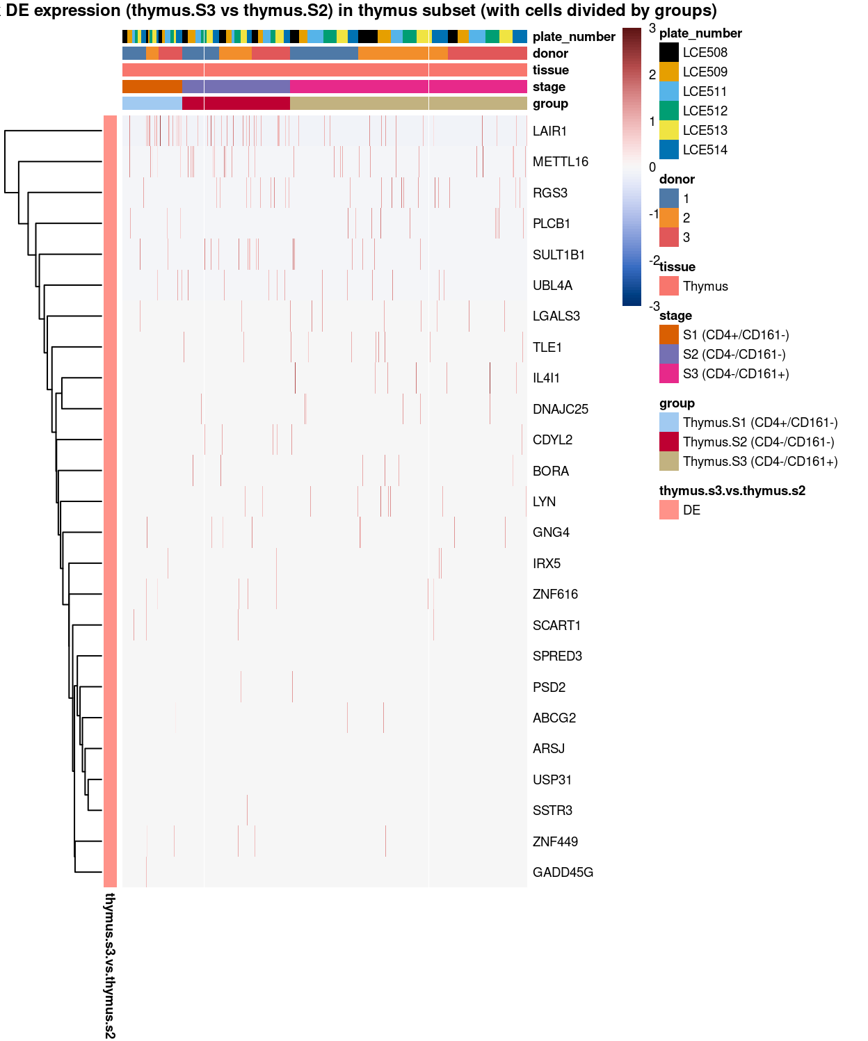
Figure 16: Heatmap of log-expression values in each sample for the marker genes identified from the mini-bulk analysis (thymus.s3.vs.thymus.s2). Cells are ordered by group. Each column is a sample, each row a gene. Colours are capped at -3 and 3 to preserve dynamic range.
Session info
Show code
sessioninfo::session_info()
─ Session info ─────────────────────────────────────────────────────
 setting  value
 version  R version 4.0.3 (2020-10-10)
 os       CentOS Linux 7 (Core)
 system   x86_64, linux-gnu
 ui       X11
 language (EN)
 collate  en_US.UTF-8
 ctype    en_US.UTF-8
 tz       Australia/Melbourne
 date     2021-09-29

─ Packages ─────────────────────────────────────────────────────────
 ! package              * version  date       lib
 P annotate               1.68.0   2020-10-27 [?]
 P AnnotationDbi          1.52.0   2020-10-27 [?]
 P assertthat             0.2.1    2019-03-21 [?]
 P batchelor            * 1.6.3    2021-04-16 [?]
 P beachmat               2.6.4    2020-12-20 [?]
 P beeswarm               0.3.1    2021-03-07 [?]
 P Biobase              * 2.50.0   2020-10-27 [?]
 P BiocGenerics         * 0.36.0   2020-10-27 [?]
 P BiocManager            1.30.12  2021-03-28 [?]
 P BiocNeighbors          1.8.2    2020-12-07 [?]
 P BiocParallel         * 1.24.1   2020-11-06 [?]
 P BiocSingular           1.6.0    2020-10-27 [?]
 P BiocStyle            * 2.18.1   2020-11-24 [?]
 P bit                    4.0.4    2020-08-04 [?]
 P bit64                  4.0.5    2020-08-30 [?]
 P bitops                 1.0-6    2013-08-17 [?]
 P blob                   1.2.1    2020-01-20 [?]
 P bluster                1.0.0    2020-10-27 [?]
 P bslib                  0.2.4    2021-01-25 [?]
 P cachem                 1.0.4    2021-02-13 [?]
 P cellranger             1.1.0    2016-07-27 [?]
 P cli                    2.4.0    2021-04-05 [?]
 P colorspace             2.0-0    2020-11-11 [?]
 P cowplot              * 1.1.1    2020-12-30 [?]
 P crayon                 1.4.1    2021-02-08 [?]
 P data.table           * 1.14.0   2021-02-21 [?]
 P DBI                    1.1.1    2021-01-15 [?]
 P DelayedArray           0.16.3   2021-03-24 [?]
 P DelayedMatrixStats     1.12.3   2021-02-03 [?]
 P DESeq2                 1.30.1   2021-02-19 [?]
 P digest                 0.6.27   2020-10-24 [?]
 P distill                1.2      2021-01-13 [?]
 P downlit                0.2.1    2020-11-04 [?]
 P dplyr                * 1.0.5    2021-03-05 [?]
 P dqrng                  0.2.1    2019-05-17 [?]
 P edgeR                * 3.32.1   2021-01-14 [?]
 P ellipsis               0.3.1    2020-05-15 [?]
 P evaluate               0.14     2019-05-28 [?]
 P fansi                  0.4.2    2021-01-15 [?]
 P farver                 2.1.0    2021-02-28 [?]
 P fastmap                1.1.0    2021-01-25 [?]
 P genefilter             1.72.1   2021-01-21 [?]
 P geneplotter            1.68.0   2020-10-27 [?]
 P generics               0.1.0    2020-10-31 [?]
 P GenomeInfoDb         * 1.26.4   2021-03-10 [?]
 P GenomeInfoDbData       1.2.4    2020-10-20 [?]
 P GenomicRanges        * 1.42.0   2020-10-27 [?]
 P ggbeeswarm             0.6.0    2017-08-07 [?]
 P ggplot2              * 3.3.3    2020-12-30 [?]
 P ggrepel              * 0.9.1    2021-01-15 [?]
 P Glimma               * 2.0.0    2020-10-27 [?]
 P glue                   1.4.2    2020-08-27 [?]
 P gridExtra              2.3      2017-09-09 [?]
 P gtable                 0.3.0    2019-03-25 [?]
 P here                 * 1.0.1    2020-12-13 [?]
 P highr                  0.9      2021-04-16 [?]
 P htmltools              0.5.1.1  2021-01-22 [?]
 P htmlwidgets            1.5.3    2020-12-10 [?]
 P httr                   1.4.2    2020-07-20 [?]
 P igraph                 1.2.6    2020-10-06 [?]
 P IRanges              * 2.24.1   2020-12-12 [?]
 P irlba                  2.3.3    2019-02-05 [?]
 P janitor              * 2.1.0    2021-01-05 [?]
 P jquerylib              0.1.3    2020-12-17 [?]
 P jsonlite               1.7.2    2020-12-09 [?]
 P knitr                  1.33     2021-04-24 [?]
 P labeling               0.4.2    2020-10-20 [?]
 P lattice                0.20-41  2020-04-02 [3]
 P lifecycle              1.0.0    2021-02-15 [?]
 P limma                * 3.46.0   2020-10-27 [?]
 P locfit                 1.5-9.4  2020-03-25 [?]
 P lubridate              1.7.10   2021-02-26 [?]
 P magrittr             * 2.0.1    2020-11-17 [?]
 P Matrix                 1.2-18   2019-11-27 [3]
 P MatrixGenerics       * 1.2.1    2021-01-30 [?]
 P matrixStats          * 0.58.0   2021-01-29 [?]
 P memoise                2.0.0    2021-01-26 [?]
 P msigdbr              * 7.2.1    2020-10-02 [?]
 P munsell                0.5.0    2018-06-12 [?]
 P patchwork            * 1.1.1    2020-12-17 [?]
 P pheatmap             * 1.0.12   2019-01-04 [?]
 P pillar                 1.5.1    2021-03-05 [?]
 P pkgconfig              2.0.3    2019-09-22 [?]
 P purrr                  0.3.4    2020-04-17 [?]
 P R.methodsS3          * 1.8.1    2020-08-26 [?]
 P R.oo                 * 1.24.0   2020-08-26 [?]
 P R.utils              * 2.10.1   2020-08-26 [?]
 P R6                     2.5.0    2020-10-28 [?]
 P RColorBrewer           1.1-2    2014-12-07 [?]
 P Rcpp                   1.0.6    2021-01-15 [?]
 P RCurl                  1.98-1.3 2021-03-16 [?]
 P readxl               * 1.3.1    2019-03-13 [?]
 P ResidualMatrix         1.0.0    2020-10-27 [?]
 P rlang                  0.4.11   2021-04-30 [?]
 P rmarkdown            * 2.7      2021-02-19 [?]
 P rprojroot              2.0.2    2020-11-15 [?]
 P RSQLite                2.2.5    2021-03-27 [?]
 P rsvd                   1.0.3    2020-02-17 [?]
 P S4Vectors            * 0.28.1   2020-12-09 [?]
 P sass                   0.3.1    2021-01-24 [?]
 P scales                 1.1.1    2020-05-11 [?]
 P scater               * 1.18.6   2021-02-26 [?]
 P scran                * 1.18.5   2021-02-04 [?]
 P scuttle                1.0.4    2020-12-17 [?]
 P sessioninfo            1.1.1    2018-11-05 [?]
 P SingleCellExperiment * 1.12.0   2020-10-27 [?]
 P snakecase              0.11.0   2019-05-25 [?]
 P sparseMatrixStats      1.2.1    2021-02-02 [?]
 P statmod                1.4.35   2020-10-19 [?]
 P stringi                1.7.3    2021-07-16 [?]
 P stringr                1.4.0    2019-02-10 [?]
 P SummarizedExperiment * 1.20.0   2020-10-27 [?]
 P survival               3.2-7    2020-09-28 [3]
 P tibble                 3.1.0    2021-02-25 [?]
 P tidyr                * 1.1.3    2021-03-03 [?]
 P tidyselect             1.1.0    2020-05-11 [?]
 P utf8                   1.2.1    2021-03-12 [?]
 P vctrs                  0.3.7    2021-03-29 [?]
 P vipor                  0.4.5    2017-03-22 [?]
 P viridis                0.5.1    2018-03-29 [?]
 P viridisLite            0.3.0    2018-02-01 [?]
 P withr                  2.4.1    2021-01-26 [?]
 P xaringanExtra          0.5.4    2021-08-04 [?]
 P xfun                   0.24     2021-06-15 [?]
 P XML                    3.99-0.6 2021-03-16 [?]
 P xtable                 1.8-4    2019-04-21 [?]
 P XVector                0.30.0   2020-10-27 [?]
 P yaml                   2.2.1    2020-02-01 [?]
 P zlibbioc               1.36.0   2020-10-27 [?]
 source
 Bioconductor
 Bioconductor
 CRAN (R 4.0.0)
 Bioconductor
 Bioconductor
 CRAN (R 4.0.3)
 Bioconductor
 Bioconductor
 CRAN (R 4.0.3)
 Bioconductor
 Bioconductor
 Bioconductor
 Bioconductor
 CRAN (R 4.0.0)
 CRAN (R 4.0.0)
 CRAN (R 4.0.0)
 CRAN (R 4.0.0)
 Bioconductor
 CRAN (R 4.0.3)
 CRAN (R 4.0.3)
 CRAN (R 4.0.0)
 CRAN (R 4.0.3)
 CRAN (R 4.0.3)
 CRAN (R 4.0.3)
 CRAN (R 4.0.3)
 CRAN (R 4.0.3)
 CRAN (R 4.0.3)
 Bioconductor
 Bioconductor
 Bioconductor
 CRAN (R 4.0.2)
 CRAN (R 4.0.3)
 CRAN (R 4.0.3)
 CRAN (R 4.0.3)
 CRAN (R 4.0.0)
 Bioconductor
 CRAN (R 4.0.0)
 CRAN (R 4.0.0)
 CRAN (R 4.0.3)
 CRAN (R 4.0.3)
 CRAN (R 4.0.3)
 Bioconductor
 Bioconductor
 CRAN (R 4.0.3)
 Bioconductor
 Bioconductor
 Bioconductor
 CRAN (R 4.0.0)
 CRAN (R 4.0.3)
 CRAN (R 4.0.3)
 Bioconductor
 CRAN (R 4.0.0)
 CRAN (R 4.0.0)
 CRAN (R 4.0.0)
 CRAN (R 4.0.3)
 CRAN (R 4.0.3)
 CRAN (R 4.0.3)
 CRAN (R 4.0.3)
 CRAN (R 4.0.0)
 CRAN (R 4.0.2)
 Bioconductor
 CRAN (R 4.0.0)
 CRAN (R 4.0.3)
 CRAN (R 4.0.3)
 CRAN (R 4.0.3)
 CRAN (R 4.0.3)
 CRAN (R 4.0.0)
 CRAN (R 4.0.3)
 CRAN (R 4.0.3)
 Bioconductor
 CRAN (R 4.0.0)
 CRAN (R 4.0.3)
 CRAN (R 4.0.3)
 CRAN (R 4.0.3)
 Bioconductor
 CRAN (R 4.0.3)
 CRAN (R 4.0.3)
 CRAN (R 4.0.2)
 CRAN (R 4.0.0)
 CRAN (R 4.0.3)
 CRAN (R 4.0.0)
 CRAN (R 4.0.3)
 CRAN (R 4.0.0)
 CRAN (R 4.0.0)
 CRAN (R 4.0.0)
 CRAN (R 4.0.0)
 CRAN (R 4.0.0)
 CRAN (R 4.0.2)
 CRAN (R 4.0.0)
 CRAN (R 4.0.3)
 CRAN (R 4.0.3)
 CRAN (R 4.0.0)
 Bioconductor
 CRAN (R 4.0.5)
 CRAN (R 4.0.3)
 CRAN (R 4.0.3)
 CRAN (R 4.0.3)
 CRAN (R 4.0.0)
 Bioconductor
 CRAN (R 4.0.3)
 CRAN (R 4.0.0)
 Bioconductor
 Bioconductor
 Bioconductor
 CRAN (R 4.0.0)
 Bioconductor
 CRAN (R 4.0.0)
 Bioconductor
 CRAN (R 4.0.2)
 CRAN (R 4.0.3)
 CRAN (R 4.0.0)
 Bioconductor
 CRAN (R 4.0.3)
 CRAN (R 4.0.3)
 CRAN (R 4.0.3)
 CRAN (R 4.0.0)
 CRAN (R 4.0.3)
 CRAN (R 4.0.3)
 CRAN (R 4.0.0)
 CRAN (R 4.0.0)
 CRAN (R 4.0.0)
 CRAN (R 4.0.3)
 Github (gadenbuie/xaringanExtra@5e2d80b)
 CRAN (R 4.0.3)
 CRAN (R 4.0.3)
 CRAN (R 4.0.0)
 Bioconductor
 CRAN (R 4.0.0)
 Bioconductor

[1] /stornext/Projects/score/Analyses/C094_Pellicci/renv/library/R-4.0/x86_64-pc-linux-gnu
[2] /tmp/RtmpP41dVI/renv-system-library
[3] /stornext/System/data/apps/R/R-4.0.3/lib64/R/library

P ── Loaded and on-disk path mismatch.Differential expression analyses is performed on the original log-expression values. We do not use the MNN-corrected values here except to obtain the clusters to be characterized.↩︎