Annotating Pellicci gamma-delta T-cell single-cell dataset (S1 and S2 only)

Show code

library(SingleCellExperiment)
library(here)
library(scater)
library(scran)
library(ggplot2)
library(cowplot)
library(edgeR)
library(Glimma)
library(BiocParallel)
library(patchwork)
library(janitor)
library(pheatmap)
library(batchelor)
library(rmarkdown)
library(BiocStyle)
library(readxl)
library(dplyr)
library(tidyr)
library(ggrepel)
library(magrittr)

knitr::opts_chunk$set(fig.path = "C094_Pellicci.single-cell.annotate.S1_S2_only_files/")

Preparing the data

We start from the cell selected SingleCellExperiment object created in ‘Merging cells for Pellicci gamma-delta T-cell dataset (S1 S2 only)’.

Show code

sce <- readRDS(here("data", "SCEs", "C094_Pellicci.single-cell.merged.S1_S2_only.SCE.rds"))

# pre-create directories for saving export, or error (dir not exists)
dir.create(here("data", "marker_genes", "S1_S2_only"), recursive = TRUE)
dir.create(here("output", "marker_genes", "S1_S2_only"), recursive = TRUE)

# Some useful colours
plate_number_colours <- setNames(
  unique(sce$colours$plate_number_colours),
  unique(names(sce$colours$plate_number_colours)))
plate_number_colours <- plate_number_colours[levels(sce$plate_number)]
tissue_colours <- setNames(
  unique(sce$colours$tissue_colours),
  unique(names(sce$colours$tissue_colours)))
tissue_colours <- tissue_colours[levels(sce$tissue)]
donor_colours <- setNames(
  unique(sce$colours$donor_colours),
  unique(names(sce$colours$donor_colours)))
donor_colours <- donor_colours[levels(sce$donor)]
stage_colours <- setNames(
  unique(sce$colours$stage_colours),
  unique(names(sce$colours$stage_colours)))
stage_colours <- stage_colours[levels(sce$stage)]
group_colours <- setNames(
  unique(sce$colours$group_colours),
  unique(names(sce$colours$group_colours)))
group_colours <- group_colours[levels(sce$group)]
cluster_colours <- setNames(
  unique(sce$colours$cluster_colours),
  unique(names(sce$colours$cluster_colours)))
cluster_colours <- cluster_colours[levels(sce$cluster)]

# Some useful gene sets
mito_set <- rownames(sce)[any(rowData(sce)$ENSEMBL.SEQNAME == "MT")]
ribo_set <- grep("^RP(S|L)", rownames(sce), value = TRUE)
# NOTE: A more curated approach for identifying ribosomal protein genes
#       (https://github.com/Bioconductor/OrchestratingSingleCellAnalysis-base/blob/ae201bf26e3e4fa82d9165d8abf4f4dc4b8e5a68/feature-selection.Rmd#L376-L380)
library(msigdbr)
c2_sets <- msigdbr(species = "Homo sapiens", category = "C2")
ribo_set <- union(
  ribo_set,
  c2_sets[c2_sets$gs_name == "KEGG_RIBOSOME", ]$gene_symbol)
ribo_set <- intersect(ribo_set, rownames(sce))
sex_set <- rownames(sce)[any(rowData(sce)$ENSEMBL.SEQNAME %in% c("X", "Y"))]
pseudogene_set <- rownames(sce)[
  any(grepl("pseudogene", rowData(sce)$ENSEMBL.GENEBIOTYPE))]
# NOTE: not suggest to narrow down into protein coding genes (pcg) as it remove all significant candidate in most of the comparison !!!
protein_coding_gene_set <- rownames(sce)[
  any(grepl("protein_coding", rowData(sce)$ENSEMBL.GENEBIOTYPE))]

Show code

# include part of the FACS data (for plot of heatmap)
facs <- t(assays(altExp(sce, "FACS"))$pseudolog)
facs_markers <- grep("V525_50_A_CD4_BV510|B530_30_A_CD161_FITC", colnames(facs), value = TRUE)
facs_selected <- facs[,facs_markers]
colnames(facs_selected) <- c("CD161", "CD4")
colData(sce) <- cbind(colData(sce), facs_selected)

Re-clustering

NOTE: Based on our explorative data analyses (EDA) on the S1 S2 only subset, we conclude the optimal number of clusters for demonstrating the heterogeneity of the dataset, we therefore re-cluster in here. Also, as indicated by Dan during our online meeting on 11 Aug 2011, we need to use different numbering and colouring for clusters in different subsets of the dataset (to prepare for publication), we perform all these by the following script.

Show code

# re-clustering
set.seed(4759)
snn_gr <- buildSNNGraph(sce, use.dimred = "corrected", k=15)
clusters <- igraph::cluster_louvain(snn_gr)
sce$cluster <- factor(clusters$membership)

# re-numbering of clusters
sce$cluster <- factor(
  dplyr::case_when(
    sce$cluster == "1" ~ "6",
    sce$cluster == "2" ~ "7",
    sce$cluster == "3" ~ "8"))

# re-colouring of clusters
cluster_colours <- setNames(
  palette.colors(nlevels(sce$cluster), "Okabe-Ito"),
  levels(sce$cluster))

After the re-clustering, there are 3 clusters for S1 S2 only subset of the dataset.

Data overview

Show code

p1 <- plotReducedDim(sce, "UMAP_corrected", colour_by = "cluster", theme_size = 7, point_size = 0.4) +
  scale_colour_manual(values = cluster_colours, name = "cluster")
p2 <- plotReducedDim(sce, "UMAP_corrected", colour_by = "stage", theme_size = 7, point_size = 0.4) +
  scale_colour_manual(values = stage_colours, name = "stage")
p3 <- plotReducedDim(sce, "UMAP_corrected", colour_by = "plate_number", theme_size = 7, point_size = 0.4) +
  scale_colour_manual(values = plate_number_colours, name = "plate_number")
p4 <- plotReducedDim(sce, "UMAP_corrected", colour_by = "tissue", theme_size = 7, point_size = 0.4) +
  scale_colour_manual(values = tissue_colours, name = "tissue")
p5 <- plotReducedDim(sce, "UMAP_corrected", colour_by = "donor", theme_size = 7, point_size = 0.4) +
  scale_colour_manual(values = donor_colours, name = "donor")
p6 <- plotReducedDim(sce, "UMAP_corrected", colour_by = "group", theme_size = 7, point_size = 0.4) +
  scale_colour_manual(values = group_colours, name = "group")
(p1 | p2) / (p3 | p4) / (p5 | p6)

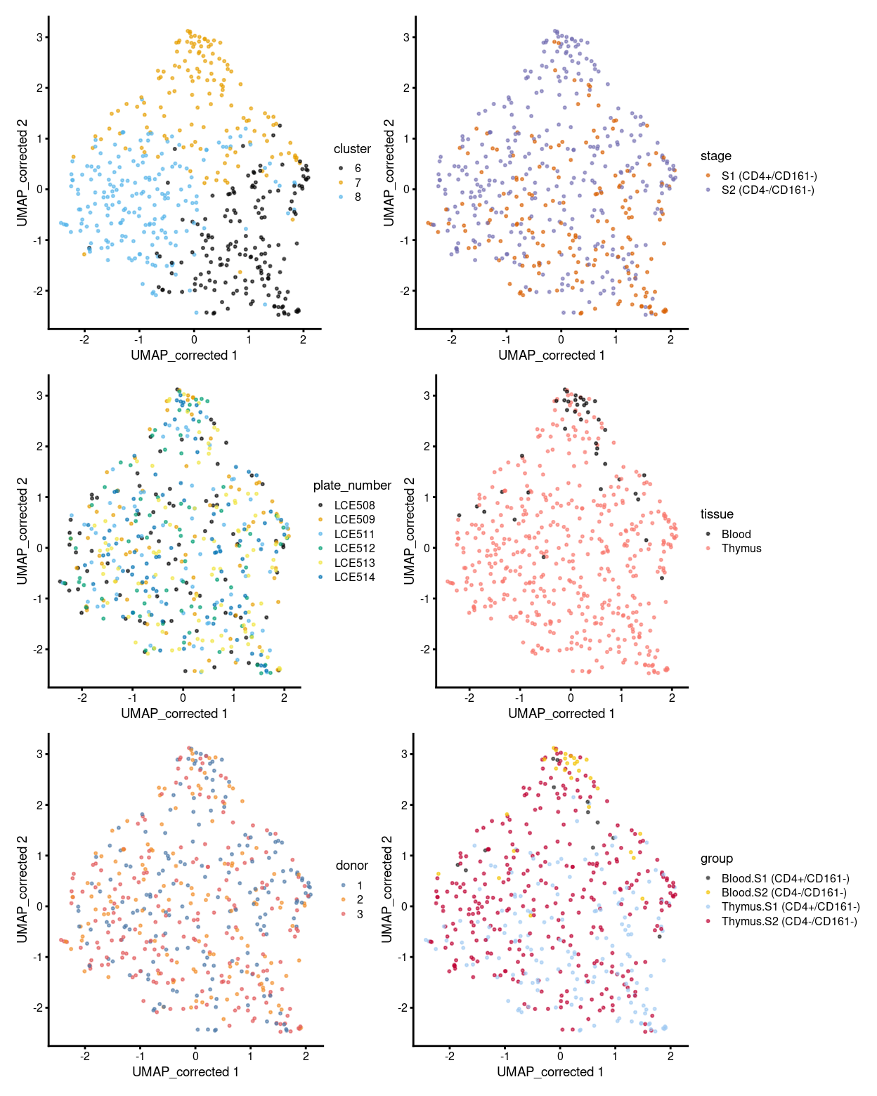
Figure 1: UMAP plot, where each point represents a cell and is coloured according to the legend.

Show code

# summary - stacked barplot
p1 <- ggcells(sce) +
  geom_bar(aes(x = cluster, fill = cluster)) +
  coord_flip() +
  ylab("Number of samples") +
  theme_cowplot(font_size = 8) +
  scale_fill_manual(values = cluster_colours) +
  geom_text(stat='count', aes(x = cluster, label=..count..), hjust=1.5, size=2)
p2 <- ggcells(sce) +
  geom_bar(
    aes(x = cluster, fill = stage),
    position = position_fill(reverse = TRUE)) +
  coord_flip() +
  ylab("Frequency") +
  scale_fill_manual(values = stage_colours) +
  theme_cowplot(font_size = 8)
p3 <- ggcells(sce) +
  geom_bar(
    aes(x = cluster, fill = plate_number),
    position = position_fill(reverse = TRUE)) +
  coord_flip() +
  ylab("Frequency") +
  scale_fill_manual(values = plate_number_colours) +
  theme_cowplot(font_size = 8)
p4 <- ggcells(sce) +
  geom_bar(
    aes(x = cluster, fill = tissue),
    position = position_fill(reverse = TRUE)) +
  coord_flip() +
  ylab("Frequency") +
  scale_fill_manual(values = tissue_colours) +
  theme_cowplot(font_size = 8)
p5 <- ggcells(sce) +
  geom_bar(
    aes(x = cluster, fill = donor),
    position = position_fill(reverse = TRUE)) +
  coord_flip() +
  ylab("Frequency") +
  scale_fill_manual(values = donor_colours) +
  theme_cowplot(font_size = 8)
p6 <- ggcells(sce) +
  geom_bar(
    aes(x = cluster, fill = group),
    position = position_fill(reverse = TRUE)) +
  coord_flip() +
  ylab("Frequency") +
  scale_fill_manual(values = group_colours) +
  theme_cowplot(font_size = 8)
(p1 | p2) / (p3 | p4) / (p5 | p6)

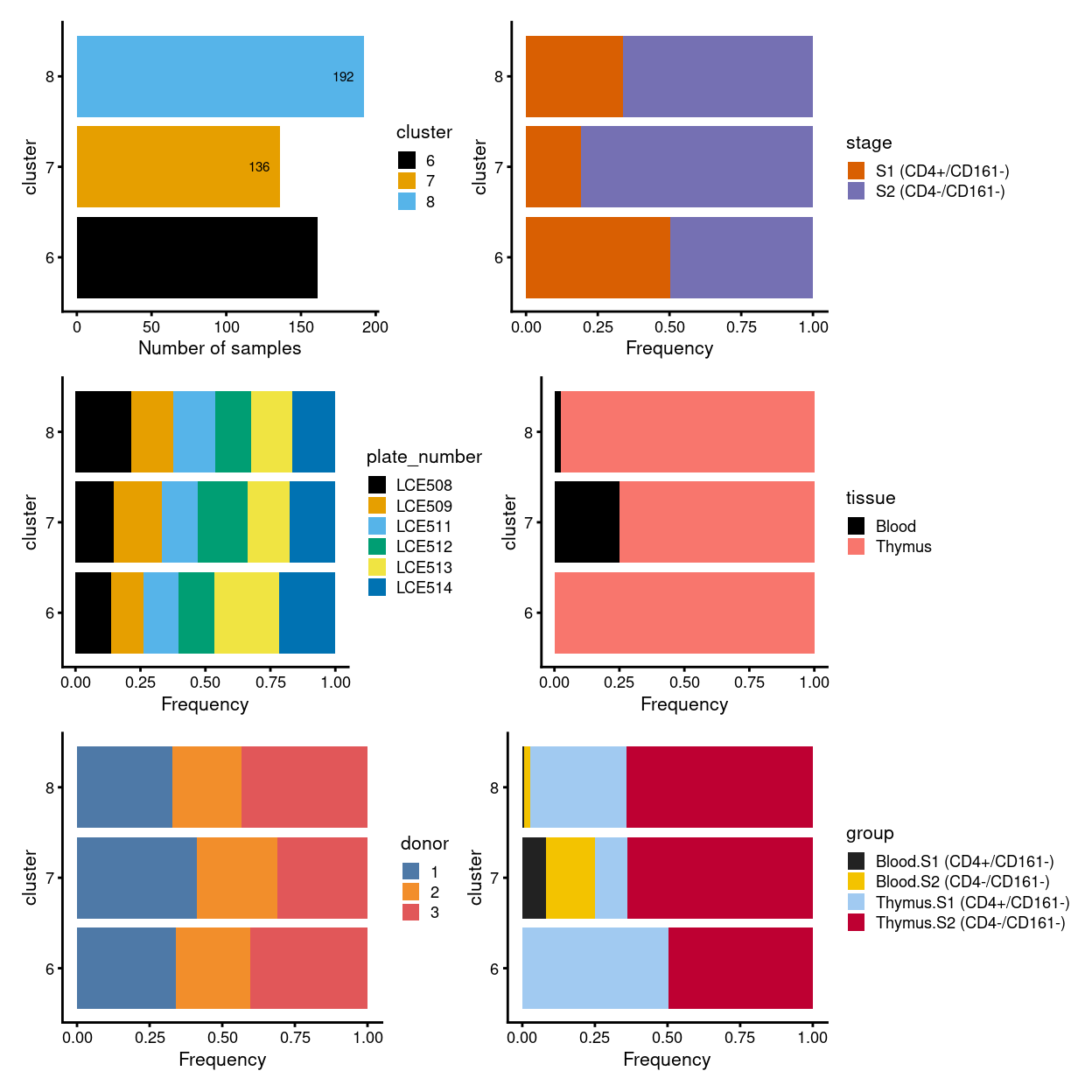
Figure 2: Breakdown of clusters by experimental factors.

NOTE: Considering the fact that SingleR with use of the annotation reference (Monaco Immune Cell Data) most relevant to the gamma-delta T cells (even annotated at cell level) could not further sub-classify the developmental stage/subtype of them (either annotating cluster as Th1 cell-/Naive CD8/CD4 T cell or Vd2gd T cells-alike) [ref: EDA_annotation_SingleR_MI_fine_cell_level.R], we decide to characterize the clusters by manual detection and curation of specific marker genes directly.

Marker gene detection

To interpret our clustering results, we identify the genes that drive separation between clusters. These marker genes allow us to assign biological meaning to each cluster based on their functional annotation. In the most obvious case, the marker genes for each cluster are a priori associated with particular cell types, allowing us to treat the clustering as a proxy for cell type identity. The same principle can be applied to more subtle differences in activation status or differentiation state.

Identification of marker genes is usually based around the retrospective detection of differential expression between clusters¹. Genes that are more strongly DE are more likely to have driven cluster separation in the first place. The top DE genes are likely to be good candidate markers as they can effectively distinguish between cells in different clusters.

The Welch t-test is an obvious choice of statistical method to test for differences in expression between clusters. It is quickly computed and has good statistical properties for large numbers of cells (Soneson and Robinson 2018).

Show code

# block on plate
sce$block <- paste0(sce$plate_number)

Cluster 6 vs. 7 vs. 8

Here we look for the unique up-regulated markers of each cluster when compared to the all remaining ones. For instance, unique markers of cluster 6 refer to the genes significantly up-regulated in all of these comparisons: cluster 7 vs. 6 and cluster 8 vs. 6.

Show code

###################################
# (M1) raw unique
#
# cluster 6 (i.e. pure.thymus.S1.S2
# cluster 7 (i.e. mostly.thymus.S1.S2.more.blood
# cluster 8 (i.e. mostly.thymus.S1.S2.less.blood

# find unique DE ./. clusters
uniquely_up <- findMarkers(
  sce,
  groups = sce$cluster,
  block = sce$block,
  pval.type = "all",
  direction = "up")

Show code

# export DGE lists
saveRDS(
  uniquely_up,
  here("data", "marker_genes", "S1_S2_only", "C094_Pellicci.uniquely_up.cluster_6_vs_7_vs_8.rds"),
  compress = "xz")

dir.create(here("output", "marker_genes", "S1_S2_only", "uniquely_up", "cluster_6_vs_7_vs_8"), recursive = TRUE)

vs_pair <- c("6", "7", "8")

message("Writing 'uniquely_up (cluster_6_vs_7_vs_8)' marker genes to file.")
for (n in names(uniquely_up)) {
  message(n)
  gzout <- gzfile(
    description = here(
      "output",
      "marker_genes",
      "S1_S2_only",
      "uniquely_up",
      "cluster_6_vs_7_vs_8",
      paste0("cluster_",
             vs_pair[which(names(uniquely_up) %in% n)],
             "_vs_",
             vs_pair[-which(names(uniquely_up) %in% n)][1],
             "_vs_",
             vs_pair[-which(names(uniquely_up) %in% n)][2],
             ".uniquely_up.csv.gz")),
    open = "wb")
  write.table(
    x = uniquely_up[[n]] %>%
      as.data.frame() %>%
      tibble::rownames_to_column("gene_ID"),
    file = gzout,
    sep = ",",
    quote = FALSE,
    row.names = FALSE,
    col.names = TRUE)
  close(gzout)
}

Show code

# NOTE: The following is a workaround to the lack of support for tabsets in 
#       distill (see https://github.com/rstudio/distill/issues/11 and 
#       https://github.com/rstudio/distill/issues/11#issuecomment-692142414 in 
#       particular).
xaringanExtra::use_panelset()

Cluster 6

Show code

##########################################
# look at cluster 6 (i.e. pure.thymus.S1.S2)
chosen <- "6"
cluster6_uniquely_up <- uniquely_up[[chosen]]

# add description for the chosen cluster-group
x <- "(pure.thymus.S1.S2)"

# look only at protein coding gene (pcg)
# NOTE: not suggest to narrow down into pcg as it remove all significant candidates (FDR << 0.05) !
# cluster6_uniquely_up <- cluster6_uniquely_up[intersect(protein_coding_gene_set, rownames(cluster6_uniquely_up)), ]

# get rid of noise (i.e. pseudo, ribo, mito, sex) that collaborator not interested in
cluster6_uniquely_up_noiseR <- cluster6_uniquely_up[setdiff(rownames(cluster6_uniquely_up), c(pseudogene_set, mito_set, ribo_set, sex_set)), ]

# see if key marker, "CD4 and/or ""KLRB1/CD161"", contain in the DE list + if it is "significant (i.e FDR <0.05)
y <- c("CD4",
       which(rownames(cluster6_uniquely_up_noiseR) %in% "CD4"),
       cluster6_uniquely_up_noiseR[which(rownames(cluster6_uniquely_up_noiseR) %in% "CD4"), ]$FDR < 0.05)
z <- c("KLRB1/CD161",
       which(rownames(cluster6_uniquely_up_noiseR) %in% "KLRB1"),
       cluster6_uniquely_up_noiseR[which(rownames(cluster6_uniquely_up_noiseR) %in% "KLRB1"), ]$FDR < 0.05)

# top25 only
best_set <- cluster6_uniquely_up_noiseR[1:25, ]

Show code

# heatmap
plotHeatmap(
  sce,
  features = rownames(best_set),
  columns = order(
    sce$cluster,
    sce$stage,
    sce$tissue,
    sce$donor,
    sce$group,
    sce$plate_number,
    sce$CD4,
    sce$CD161),
  colour_columns_by = c(
    "cluster",
    "stage",
    "tissue",
    "donor",
    "group",
    "plate_number",
    "CD4",
    "CD161"),
  cluster_cols = FALSE,
  center = TRUE,
  symmetric = TRUE,
  zlim = c(-3, 3),
  show_colnames = FALSE,
  annotation_row = data.frame(
    Sig = factor(
      ifelse(best_set[, "FDR"] < 0.05, "Yes", "No"),
      # TODO: temp trick to deal with the row-colouring problem
      # levels = c("Yes", "No")),
      levels = c("Yes")),
    row.names = rownames(best_set)),
  main = paste0("Cluster ", chosen, " ", x, " - \n",
                y[1], "_top ", y[2], "_significance: ", y[3], " ; \n",
                z[1], "_top ", z[2], "_significance: ", z[3]),
  column_annotation_colors = list(
    # Sig = c("Yes" = "red", "No" = "lightgrey"),
    cluster = cluster_colours,
    stage = stage_colours,
    tissue = tissue_colours,
    donor = donor_colours,
    group = group_colours,
    plate_number = plate_number_colours),
  color = hcl.colors(101, "Blue-Red 3"),
  fontsize = 7)

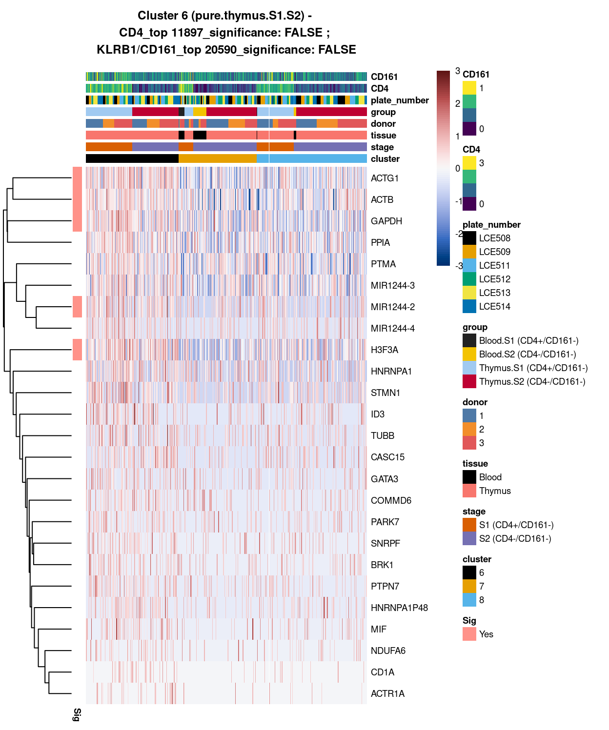
Figure 3: Heatmap of log-expression values in each sample for the top uniquely upregulated marker genes. Each column is a sample, each row a gene. Colours are capped at -3 and 3 to preserve dynamic range. Ranking of CD4 and CD161/KLRB1 from top of the DGE list sorted in ascending order of FDR and their statistical significance (TRUE = FDR < 0.05) are provided in the title

Cluster 7

Show code

##########################################
# look at cluster 7 (i.e. S3.mix.with.blood.1)
chosen <- "7"
cluster7_uniquely_up <- uniquely_up[[chosen]]

# add description for the chosen cluster-group
x <- "(mostly.thymus.S1.S2.more.blood)"

# look only at protein coding gene (pcg)
# NOTE: not suggest to narrow down into pcg as it remove all significant candidates (FDR << 0.05) !
# cluster7_uniquely_up <- cluster7_uniquely_up[intersect(protein_coding_gene_set, rownames(cluster7_uniquely_up)), ]

# get rid of noise (i.e. pseudo, ribo, mito, sex) that collaborator not interested in
cluster7_uniquely_up_noiseR <- cluster7_uniquely_up[setdiff(rownames(cluster7_uniquely_up), c(pseudogene_set, mito_set, ribo_set, sex_set)), ]

# see if key marker, "CD4 and/or ""KLRB1/CD161"", contain in the DE list + if it is "significant (i.e FDR <0.05)
y <- c("CD4",
       which(rownames(cluster7_uniquely_up_noiseR) %in% "CD4"),
       cluster7_uniquely_up_noiseR[which(rownames(cluster7_uniquely_up_noiseR) %in% "CD4"), ]$FDR < 0.05)
z <- c("KLRB1/CD161",
       which(rownames(cluster7_uniquely_up_noiseR) %in% "KLRB1"),
       cluster7_uniquely_up_noiseR[which(rownames(cluster7_uniquely_up_noiseR) %in% "KLRB1"), ]$FDR < 0.05)

# top25 only
best_set <- cluster7_uniquely_up_noiseR[1:25, ]

Show code

# heatmap
plotHeatmap(
  sce,
  features = rownames(best_set),
  columns = order(
    sce$cluster,
    sce$stage,
    sce$tissue,
    sce$donor,
    sce$group,
    sce$plate_number,
    sce$CD4,
    sce$CD161),
  colour_columns_by = c(
    "cluster",
    "stage",
    "tissue",
    "donor",
    "group",
    "plate_number",
    "CD4",
    "CD161"),
  cluster_cols = FALSE,
  center = TRUE,
  symmetric = TRUE,
  zlim = c(-3, 3),
  show_colnames = FALSE,
  annotation_row = data.frame(
    Sig = factor(
      ifelse(best_set[, "FDR"] < 0.05, "Yes", "No"),
      # TODO: temp trick to deal with the row-colouring problem
      # levels = c("Yes", "No")),
      levels = c("Yes")),
    row.names = rownames(best_set)),
  main = paste0("Cluster ", chosen, " ", x, " - \n",
                y[1], "_top ", y[2], "_significance: ", y[3], " ; \n",
                z[1], "_top ", z[2], "_significance: ", z[3]),
  column_annotation_colors = list(
    # Sig = c("Yes" = "red", "No" = "lightgrey"),
    cluster = cluster_colours,
    stage = stage_colours,
    tissue = tissue_colours,
    donor = donor_colours,
    group = group_colours,
    plate_number = plate_number_colours),
  color = hcl.colors(101, "Blue-Red 3"),
  fontsize = 7)

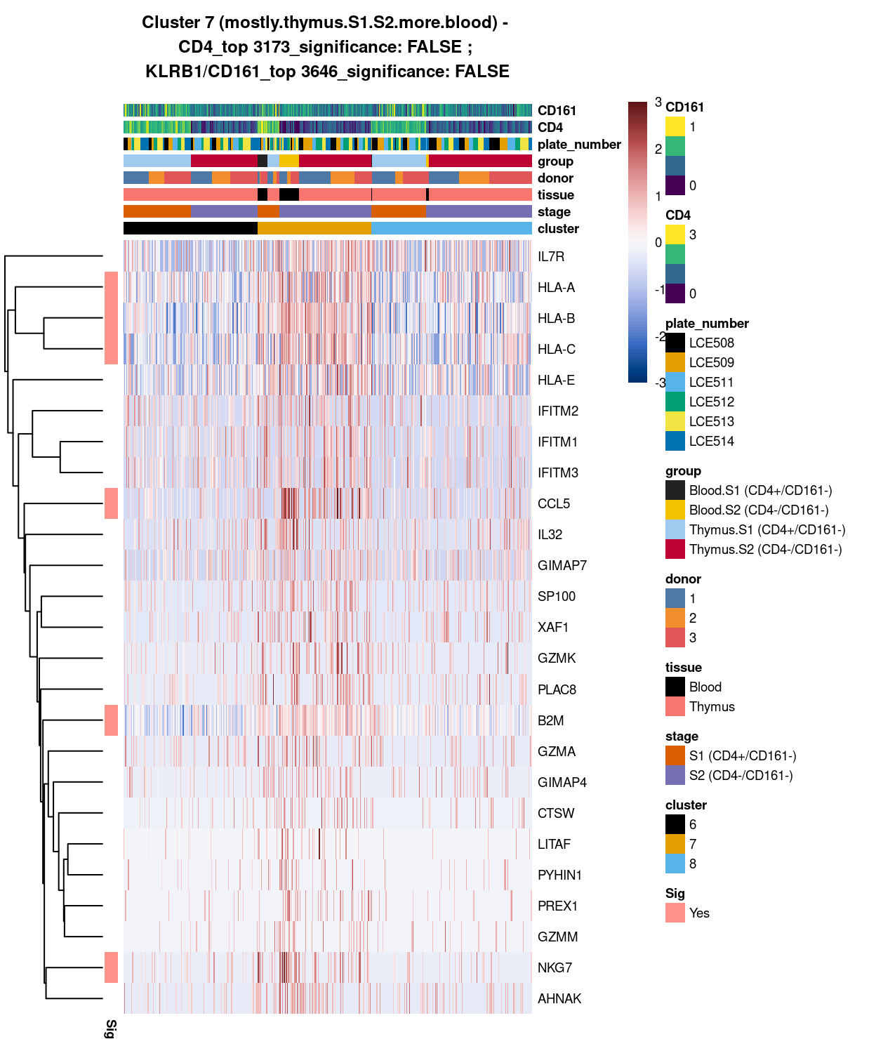
Figure 4: Heatmap of log-expression values in each sample for the top uniquely upregulated marker genes. Each column is a sample, each row a gene. Colours are capped at -3 and 3 to preserve dynamic range. Ranking of CD4 and CD161/KLRB1 from top of the DGE list sorted in ascending order of FDR and their statistical significance (TRUE = FDR < 0.05) are provided in the title

Cluster 8

Show code

##########################################
# look at cluster 8 (i.e. mostly.thymus.S1.S2.less.blood)
chosen <- "8"
cluster8_uniquely_up <- uniquely_up[[chosen]]

# add description for the chosen cluster-group
x <- "(mostly.thymus.S1.S2.less.blood)"

# look only at protein coding gene (pcg)
# NOTE: not suggest to narrow down into pcg as it remove all significant candidates (FDR << 0.05) !
# cluster8_uniquely_up <- cluster8_uniquely_up[intersect(protein_coding_gene_set, rownames(cluster8_uniquely_up)), ]

# get rid of noise (i.e. pseudo, ribo, mito, sex) that collaborator not interested in
cluster8_uniquely_up_noiseR <- cluster8_uniquely_up[setdiff(rownames(cluster8_uniquely_up), c(pseudogene_set, mito_set, ribo_set, sex_set)), ]

# see if key marker, "CD4 and/or ""KLRB1/CD161"", contain in the DE list + if it is "significant (i.e FDR <0.05)
y <- c("CD4",
       which(rownames(cluster8_uniquely_up_noiseR) %in% "CD4"),
       cluster8_uniquely_up_noiseR[which(rownames(cluster8_uniquely_up_noiseR) %in% "CD4"), ]$FDR < 0.05)
z <- c("KLRB1/CD161",
       which(rownames(cluster8_uniquely_up_noiseR) %in% "KLRB1"),
       cluster8_uniquely_up_noiseR[which(rownames(cluster8_uniquely_up_noiseR) %in% "KLRB1"), ]$FDR < 0.05)

# top25 only
best_set <- cluster8_uniquely_up_noiseR[1:25, ]

Show code

# heatmap
plotHeatmap(
  sce,
  features = rownames(best_set),
  columns = order(
    sce$cluster,
    sce$stage,
    sce$tissue,
    sce$donor,
    sce$group,
    sce$plate_number,
    sce$CD4,
    sce$CD161),
  colour_columns_by = c(
    "cluster",
    "stage",
    "tissue",
    "donor",
    "group",
    "plate_number",
    "CD4",
    "CD161"),
  cluster_cols = FALSE,
  center = TRUE,
  symmetric = TRUE,
  zlim = c(-3, 3),
  show_colnames = FALSE,
  # annotation_row = data.frame(
  #   Sig = factor(
  #     ifelse(best_set[, "FDR"] < 0.05, "Yes", "No"),
  #     # TODO: temp trick to deal with the row-colouring problem
  #     # levels = c("Yes", "No")),
  #     levels = c("Yes")),
  #   row.names = rownames(best_set)),
  main = paste0("Cluster ", chosen, " ", x, " - \n",
                y[1], "_top ", y[2], "_significance: ", y[3], " ; \n",
                z[1], "_top ", z[2], "_significance: ", z[3]),
  column_annotation_colors = list(
    # Sig = c("Yes" = "red", "No" = "lightgrey"),
    cluster = cluster_colours,
    stage = stage_colours,
    tissue = tissue_colours,
    donor = donor_colours,
    group = group_colours,
    plate_number = plate_number_colours),
  color = hcl.colors(101, "Blue-Red 3"),
  fontsize = 7)

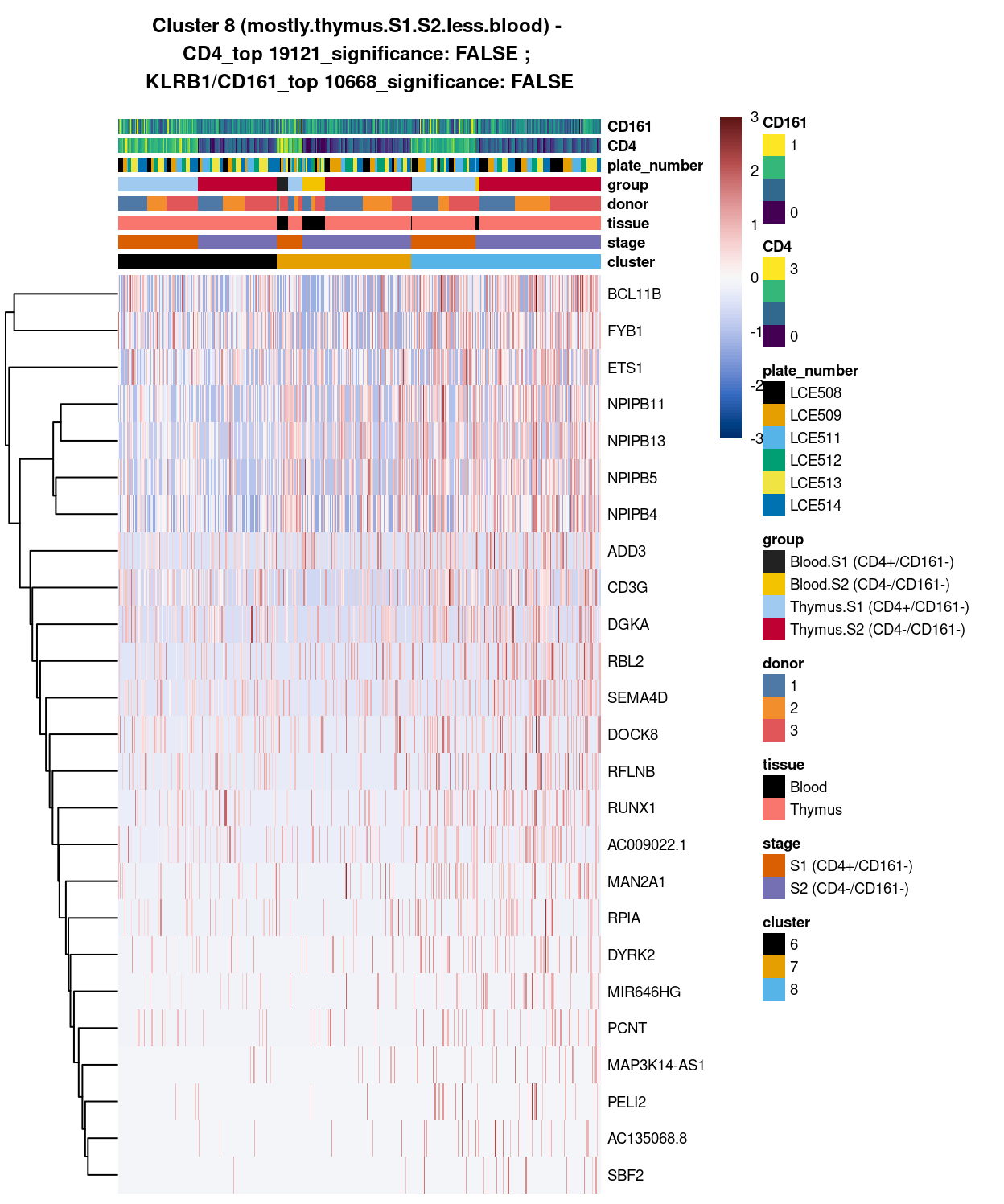
Figure 5: Heatmap of log-expression values in each sample for the top uniquely upregulated marker genes. Each column is a sample, each row a gene. Colours are capped at -3 and 3 to preserve dynamic range. Ranking of CD4 and CD161/KLRB1 from top of the DGE list sorted in ascending order of FDR and their statistical significance (TRUE = FDR < 0.05) are provided in the title

DGE lists of these comparisons are available in output/marker_genes/S1_S2_only/uniquely_up/cluster_6_vs_7_vs_8/.

Summary:

Except for cluster 8 (mostly.thymus.S1.S2.less.blood) , both cluster 6 and 7 already show number of globally unique markers. For instance, cluster 6 (i.e. pure.thymus.S1.S2) shows clear up-regulation of ACTG1, ACTB, GAPDH, MIR1244-2 and H3F3A expression compared to cluster 7 and 8. Whilst Cluster 7 (i.e. mostly.thymus.S1.S2.more.blood) also demonstrate unique increase in gene expression such as of class I HLA, CCL5, NKG7, and B2M (in which CCL5 expression seem to be relatively higher in blood.S2, whilst NKG7 expression are relatively higher in both S1 and 2 of blood cells). From these, it is apparent that at least cluster 6 and 7 are different clusters (whilst for cluster 8, its uniqueness could be shown in selected pairwise comparison).

With this regard, apart from making “all pairwise comparisons” between “all clusters” to pinpoint DE unique to each cluster as above, we took an alternative path and determined the DE unique to only the “selected pairwise comparisons” between “clusters” below. Say, for cluster 8, we determine markers that is significantly up-regulated in at least one of these comparisons: cluster 6 vs. 8 or cluster 7 vs. 8.

Besides, we also look into the pairwise comparisons between the interesting “cluster-groups.” For instance, cluster 6 is the only cluster with pure thymus origin. It would be interesting to know how cluster 6 is different from both cluster 7 and 8, which is a S1-S2-mix of thymus cells with varying amount of blood cells.

Here are the list of pairwise comparisons and what they are anticipated to achieve when compared:

fx: how is thymus.S1.S2 cells with blood are different from pure thymus.S1.S2 cells

• 7 vs 6 (A vs B)
• 8 vs 6 (C vs D)
• 7_8 vs 6 (E vs F)

fx: how is thymus.S1.S2 cells with more blood are different from thymus.S1.S2 cells with less blood

• 7 vs 8 (G vs H)

Selected pairwise comparisons

Show code

# NOTE: The following is a workaround to the lack of support for tabsets in 
#       distill (see https://github.com/rstudio/distill/issues/11 and 
#       https://github.com/rstudio/distill/issues/11#issuecomment-692142414 in 
#       particular).
xaringanExtra::use_panelset()

cluster_7_vs_cluster_6

Show code

#########
# A vs B
#########

##########################################################################################
# cluster 7 (i.e. mostly.thymus.S1.S2.more.blood) vs cluster 6 (i.e. pure.thymus.S1.S2)

# checkpoint
cp <- sce
# exclude cells of uninterested cluster from cp
cp <- cp[, cp$cluster == "7" | cp$cluster == "6"]
colData(cp) <- droplevels(colData(cp))

# classify cluster-group for comparison
cp$vs1 <- factor(ifelse(cp$cluster == 7, "A", "B"))

# set vs colours
vs1_colours <- setNames(
  palette.colors(nlevels(cp$vs1), "Set1"),
  levels(cp$vs1))
cp$colours$vs1_colours <- vs1_colours[cp$vs1]

# find unique DE ./. cluster-groups
vs1_uniquely_up <- findMarkers(
  cp,
  groups = cp$vs1,
  block = cp$block,
  pval.type = "all",
  direction = "up")

# export DGE lists
saveRDS(
  vs1_uniquely_up,
  here("data", "marker_genes", "S1_S2_only", "C094_Pellicci.uniquely_up.cluster_7_vs_6.rds"),
  compress = "xz")

dir.create(here("output", "marker_genes", "S1_S2_only", "uniquely_up", "cluster_7_vs_6"), recursive = TRUE)

vs_pair <- c("7", "6")

message("Writing 'uniquely_up (cluster_7_vs_6)' marker genes to file.")
for (n in names(vs1_uniquely_up)) {
  message(n)
  gzout <- gzfile(
    description = here(
      "output",
      "marker_genes",
      "S1_S2_only",
      "uniquely_up",
      "cluster_7_vs_6",
      paste0("cluster_",
             vs_pair[which(names(vs1_uniquely_up) %in% n)],
             "_vs_",
             vs_pair[-which(names(vs1_uniquely_up) %in% n)][1],
             ".uniquely_up.csv.gz")),
    open = "wb")
  write.table(
    x = vs1_uniquely_up[[n]] %>%
      as.data.frame() %>%
      tibble::rownames_to_column("gene_ID"),
    file = gzout,
    sep = ",",
    quote = FALSE,
    row.names = FALSE,
    col.names = TRUE)
  close(gzout)
}

Show code

###############################################################
# look at cluster-group A / cluster 7 (i.e. mostly.thymus.S1.S2.more.blood)
chosen <- "A"
A_uniquely_up <- vs1_uniquely_up[[chosen]]

# add description for the chosen cluster-group
x <- "(cluster 7; mostly.thymus.S1.S2.more.blood)"

# look only at protein coding gene (pcg)
# NOTE: not suggest to narrow down into pcg as it remove all significant candidates (FDR << 0.05) !
# A_uniquely_up_pcg <- A_uniquely_up[intersect(protein_coding_gene_set, rownames(A_uniquely_up)), ]

# get rid of noise (i.e. pseudo, ribo, mito, sex) that collaborator not interested in
A_uniquely_up_noiseR <- A_uniquely_up[setdiff(rownames(A_uniquely_up), c(pseudogene_set, mito_set, ribo_set, sex_set)), ]

# see if key marker, "CD4 and/or ""KLRB1/CD161"", contain in the DE list + if it is "significant (i.e FDR <0.05)
y <- c("CD4",
       which(rownames(A_uniquely_up_noiseR) %in% "CD4"),
       A_uniquely_up_noiseR[which(rownames(A_uniquely_up_noiseR) %in% "CD4"), ]$FDR < 0.05)
z <- c("KLRB1/CD161",
       which(rownames(A_uniquely_up_noiseR) %in% "KLRB1"),
       A_uniquely_up_noiseR[which(rownames(A_uniquely_up_noiseR) %in% "KLRB1"), ]$FDR < 0.05)

# top25 only + gene-of-interest
best_set <- A_uniquely_up_noiseR[1:25, ]

Show code

# heatmap
plotHeatmap(
  cp,
  features = rownames(best_set),
  columns = order(
    cp$vs1,
    cp$cluster,
    cp$stage,
    cp$tissue,
    cp$donor,
    cp$group,
    cp$plate_number,
    cp$CD4,
    cp$CD161),
  colour_columns_by = c(
    "vs1",
    "cluster",
    "stage",
    "tissue",
    "donor",
    "group",
    "plate_number",
    "CD4",
    "CD161"),
  cluster_cols = FALSE,
  center = TRUE,
  symmetric = TRUE,
  zlim = c(-3, 3),
  show_colnames = FALSE,
  annotation_row = data.frame(
    Sig = factor(
      ifelse(best_set[, "FDR"] < 0.05, "Yes", "No"),
      # TODO: temp trick to deal with the row-colouring problem
      # levels = c("Yes", "No")),
      levels = c("Yes")),
    row.names = rownames(best_set)),
  main = paste0("Cluster-group: ", chosen, " ", x, " - \n",
                y[1], "_top ", y[2], "_significance: ", y[3], " ; \n",
                z[1], "_top ", z[2], "_significance: ", z[3]),
  column_annotation_colors = list(
    # Sig = c("Yes" = "red", "No" = "lightgrey"),
    vs1 = vs1_colours,
    cluster = cluster_colours,
    stage = stage_colours,
    tissue = tissue_colours,
    donor = donor_colours,
    group = group_colours,
    plate_number = plate_number_colours),
  color = hcl.colors(101, "Blue-Red 3"),
  fontsize = 7)

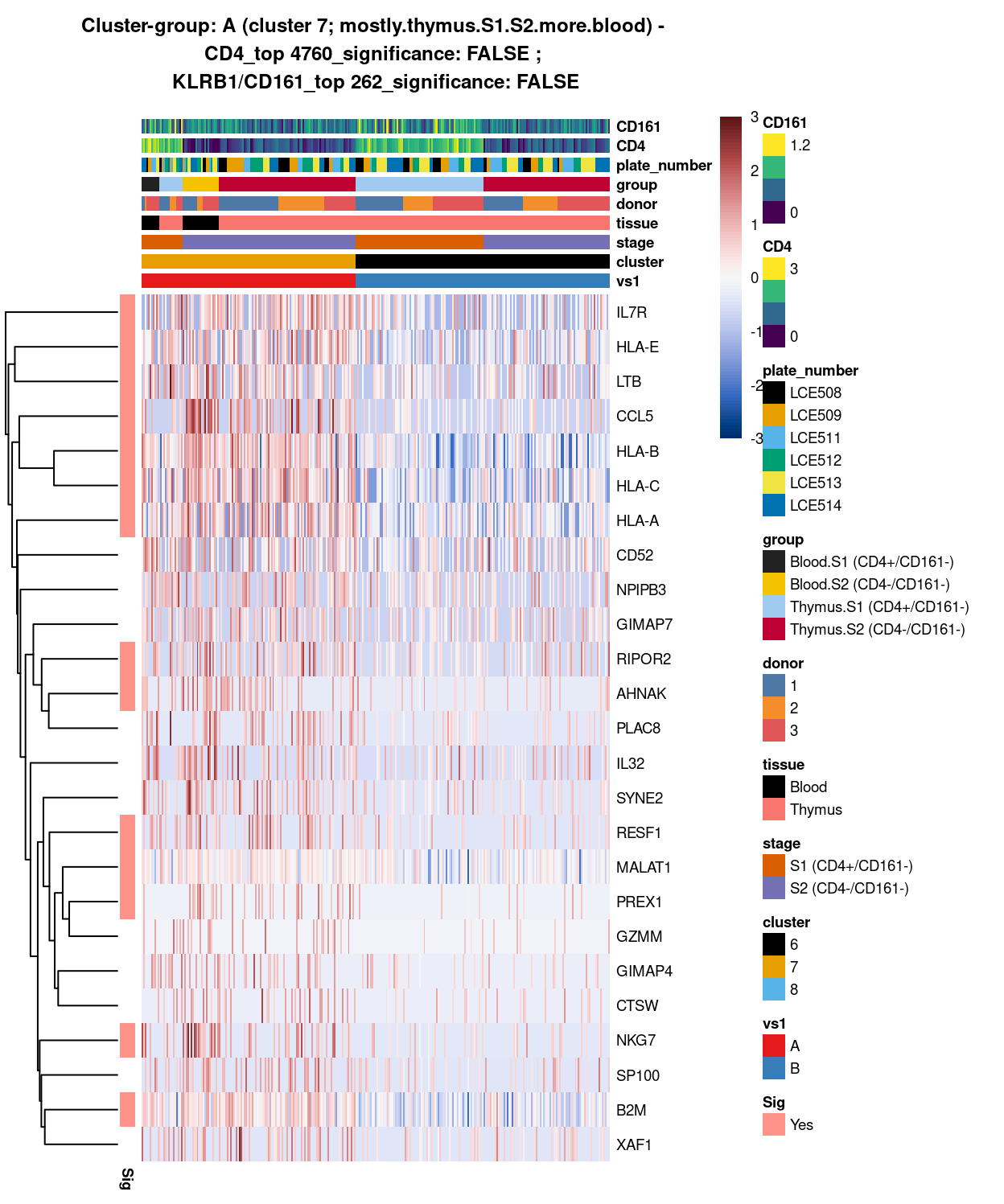
Figure 6: Heatmap of log-expression values in each sample for the top uniquely upregulated marker genes. Each column is a sample, each row a gene. Colours are capped at -3 and 3 to preserve dynamic range. Ranking of CD4 and CD161/KLRB1 from top of the DGE list sorted in ascending order of FDR and their statistical significance (TRUE = FDR < 0.05) are provided in the title.

Show code

##########################################################
# look at cluster-group B / cluster 6 (i.e. pure.thymus.S1.S2)
chosen <- "B"
B_uniquely_up <- vs1_uniquely_up[[chosen]]

# add description for the chosen cluster-group
x <- "(cluster 6; pure.thymus.S1.S2)"

# look only at protein coding gene (pcg)
# NOTE: not suggest to narrow down into pcg as it remove all significant candidates (FDR << 0.05) !
# B_uniquely_up_pcg <- B_uniquely_up[intersect(protein_coding_gene_set, rownames(B_uniquely_up)), ]

# get rid of noise (i.e. pseudo, ribo, mito, sex) that collaborator not interested in
B_uniquely_up_noiseR <- B_uniquely_up[setdiff(rownames(B_uniquely_up), c(pseudogene_set, mito_set, ribo_set, sex_set)), ]

# see if key marker, "CD4 and/or ""KLRB1/CD161"", contain in the DE list + if it is "significant (i.e FDR <0.05)
y <- c("CD4",
       which(rownames(B_uniquely_up_noiseR) %in% "CD4"),
       B_uniquely_up_noiseR[which(rownames(B_uniquely_up_noiseR) %in% "CD4"), ]$FDR < 0.05)
z <- c("KLRB1/CD161",
       which(rownames(B_uniquely_up_noiseR) %in% "KLRB1"),
       B_uniquely_up_noiseR[which(rownames(B_uniquely_up_noiseR) %in% "KLRB1"), ]$FDR < 0.05)

# top25 only + gene-of-interest
best_set <- B_uniquely_up_noiseR[1:25, ]

Show code

# heatmap
plotHeatmap(
  cp,
  features = rownames(best_set),
  columns = order(
    cp$vs1,
    cp$cluster,
    cp$stage,
    cp$tissue,
    cp$donor,
    cp$group,
    cp$plate_number,
    cp$CD4,
    cp$CD161),
  colour_columns_by = c(
    "vs1",
    "cluster",
    "stage",
    "tissue",
    "donor",
    "group",
    "plate_number",
    "CD4",
    "CD161"),
  cluster_cols = FALSE,
  center = TRUE,
  symmetric = TRUE,
  zlim = c(-3, 3),
  show_colnames = FALSE,
  annotation_row = data.frame(
    Sig = factor(
      ifelse(best_set[, "FDR"] < 0.05, "Yes", "No"),
      # TODO: temp trick to deal with the row-colouring problem
      # levels = c("Yes", "No")),
      levels = c("Yes")),
    row.names = rownames(best_set)),
  main = paste0("Cluster-group: ", chosen, " ", x, " - \n",
                y[1], "_top ", y[2], "_significance: ", y[3], " ; \n",
                z[1], "_top ", z[2], "_significance: ", z[3]),
  column_annotation_colors = list(
    # Sig = c("Yes" = "red", "No" = "lightgrey"),
    vs1 = vs1_colours,
    cluster = cluster_colours,
    stage = stage_colours,
    tissue = tissue_colours,
    donor = donor_colours,
    group = group_colours,
    plate_number = plate_number_colours),
  color = hcl.colors(101, "Blue-Red 3"),
  fontsize = 7)

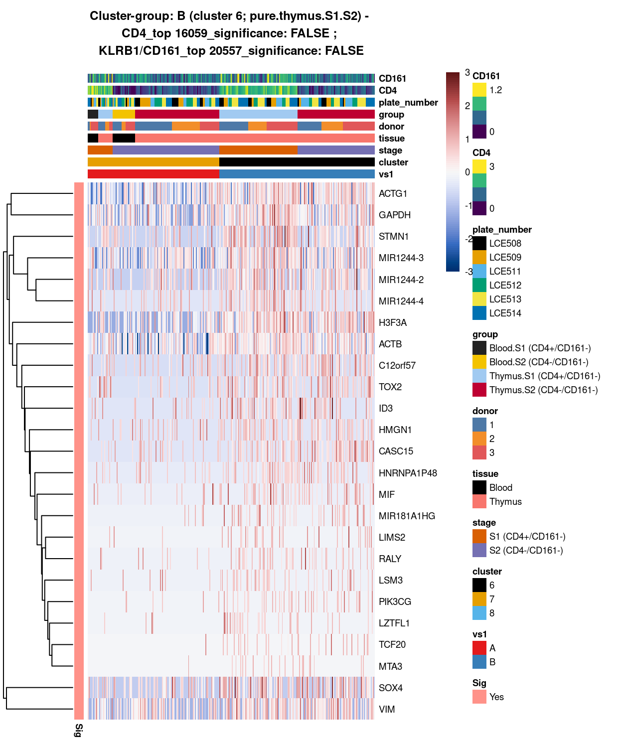
Figure 7: Heatmap of log-expression values in each sample for the top uniquely upregulated marker genes. Each column is a sample, each row a gene. Colours are capped at -3 and 3 to preserve dynamic range. Ranking of CD4 and CD161/KLRB1 from top of the DGE list sorted in ascending order of FDR and their statistical significance (TRUE = FDR < 0.05) are provided in the title.

DGE lists of these comparisons are available in output/marker_genes/S1_S2_only/uniquely_up/cluster_7_vs_6/.

SUMMARY: 7 vs 6 (A vs B)

• cluster 7 (mostly.thymus.S1.S2.more.blood >>> number of unique marker found (say, IL7R, , LTB, CCL5, NKG7. etc)
• cluster 6 (pure.thymus.S1.S2 >>> lots of marker up-regulated in cluster 1; in which, say STMN1 and MIR1244-4, seems to be more highly expression in S1 than S2
• COMMENT: cluster 1 and 2 are 2 separated clusters

cluster_8_vs_cluster_6

Show code

#########
# C vs D
#########

##########################################################################################
# cluster 8 (i.e. mostly.thymus.S1.S2.less.blood) vs cluster 6 (i.e. pure.thymus.S1.S2)

# checkpoint
cp <- sce
# exclude cells of uninterested cluster from cp
cp <- cp[, cp$cluster == "8" | cp$cluster == "6"]
colData(cp) <- droplevels(colData(cp))

# classify cluster-group for comparison
cp$vs2 <- factor(ifelse(cp$cluster == 8, "C", "D"))

# set vs colours
vs2_colours <- setNames(
  palette.colors(nlevels(cp$vs2), "Set1"),
  levels(cp$vs2))
cp$colours$vs2_colours <- vs2_colours[cp$vs2]

# find unique DE ./. cluster-groups
vs2_uniquely_up <- findMarkers(
  cp,
  groups = cp$vs2,
  block = cp$block,
  pval.type = "all",
  direction = "up")

# export DGE lists
saveRDS(
  vs2_uniquely_up,
  here("data", "marker_genes", "S1_S2_only", "C094_Pellicci.uniquely_up.cluster_8_vs_6.rds"),
  compress = "xz")

dir.create(here("output", "marker_genes", "S1_S2_only", "uniquely_up", "cluster_8_vs_6"), recursive = TRUE)

vs_pair <- c("8", "6")

message("Writing 'uniquely_up (cluster_8_vs_6)' marker genes to file.")
for (n in names(vs2_uniquely_up)) {
  message(n)
  gzout <- gzfile(
    description = here(
      "output",
      "marker_genes",
      "S1_S2_only",
      "uniquely_up",
      "cluster_8_vs_6",
      paste0("cluster_",
             vs_pair[which(names(vs2_uniquely_up) %in% n)],
             "_vs_",
             vs_pair[-which(names(vs2_uniquely_up) %in% n)][1],
             ".uniquely_up.csv.gz")),
    open = "wb")
  write.table(
    x = vs2_uniquely_up[[n]] %>%
      as.data.frame() %>%
      tibble::rownames_to_column("gene_ID"),
    file = gzout,
    sep = ",",
    quote = FALSE,
    row.names = FALSE,
    col.names = TRUE)
  close(gzout)
}

Show code

###############################################################
# look at cluster-group C / cluster 8 (i.e. mostly.thymus.S1.S2.less.blood)
chosen <- "C"
C_uniquely_up <- vs2_uniquely_up[[chosen]]

# add description for the chosen cluster-group
x <- "(cluster 8; mostly.thymus.S1.S2.less.blood)"

# look only at protein coding gene (pcg)
# NOTE: not suggest to narrow down into pcg as it remove all significant candidates (FDR << 0.05) !
# C_uniquely_up_pcg <- C_uniquely_up[intersect(protein_coding_gene_set, rownames(C_uniquely_up)), ]

# get rid of noise (i.e. pseudo, ribo, mito, sex) that collaborator not interested in
C_uniquely_up_noiseR <- C_uniquely_up[setdiff(rownames(C_uniquely_up), c(pseudogene_set, mito_set, ribo_set, sex_set)), ]

# see if key marker, "CD4 and/or ""KLRB1/CD161"", contain in the DE list + if it is "significant (i.e FDR <0.05)
y <- c("CD4",
       which(rownames(C_uniquely_up_noiseR) %in% "CD4"),
       C_uniquely_up_noiseR[which(rownames(C_uniquely_up_noiseR) %in% "CD4"), ]$FDR < 0.05)
z <- c("KLRB1/CD161",
       which(rownames(C_uniquely_up_noiseR) %in% "KLRB1"),
       C_uniquely_up_noiseR[which(rownames(C_uniquely_up_noiseR) %in% "KLRB1"), ]$FDR < 0.05)

# top25 only + gene-of-interest
best_set <- C_uniquely_up_noiseR[1:25, ]

Show code

# heatmap
plotHeatmap(
  cp,
  features = rownames(best_set),
  columns = order(
    cp$vs2,
    cp$cluster,
    cp$stage,
    cp$tissue,
    cp$donor,
    cp$group,
    cp$plate_number,
    cp$CD4,
    cp$CD161),
  colour_columns_by = c(
    "vs2",
    "cluster",
    "stage",
    "tissue",
    "donor",
    "group",
    "plate_number",
    "CD4",
    "CD161"),
  cluster_cols = FALSE,
  center = TRUE,
  symmetric = TRUE,
  zlim = c(-3, 3),
  show_colnames = FALSE,
  annotation_row = data.frame(
    Sig = factor(
      ifelse(best_set[, "FDR"] < 0.05, "Yes", "No"),
      # TODO: temp trick to deal with the row-colouring problem
      # levels = c("Yes", "No")),
      levels = c("Yes")),
    row.names = rownames(best_set)),
  main = paste0("Cluster-group: ", chosen, " ", x, " - \n",
                y[1], "_top ", y[2], "_significance: ", y[3], " ; \n",
                z[1], "_top ", z[2], "_significance: ", z[3]),
  column_annotation_colors = list(
    # Sig = c("Yes" = "red", "No" = "lightgrey"),
    vs2 = vs2_colours,
    cluster = cluster_colours,
    stage = stage_colours,
    tissue = tissue_colours,
    donor = donor_colours,
    group = group_colours,
    plate_number = plate_number_colours),
  color = hcl.colors(101, "Blue-Red 3"),
  fontsize = 7)

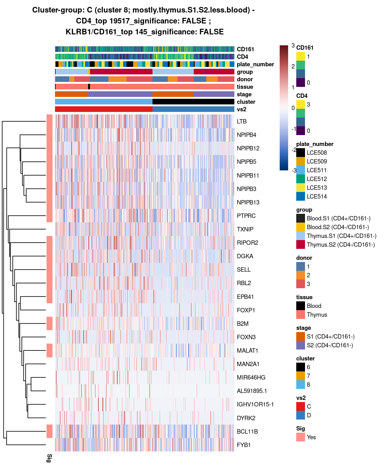
Figure 8: Heatmap of log-expression values in each sample for the top uniquely upregulated marker genes. Each column is a sample, each row a gene. Colours are capped at -3 and 3 to preserve dynamic range. Ranking of CD4 and CD161/KLRB1 from top of the DGE list sorted in ascending order of FDR and their statistical significance (TRUE = FDR < 0.05) are provided in the title.

Show code

##########################################################
# look at cluster-group D / cluster 6 (i.e. pure.thymus.S1.S2)
chosen <- "D"
D_uniquely_up <- vs2_uniquely_up[[chosen]]

# add description for the chosen cluster-group
x <- "(cluster 6; pure.thymus.S1.S2)"

# look only at protein coding gene (pcg)
# NOTE: not suggest to narrow down into pcg as it remove all significant candidates (FDR << 0.05) !
# D_uniquely_up_pcg <- D_uniquely_up[intersect(protein_coding_gene_set, rownames(D_uniquely_up)), ]

# get rid of noise (i.e. pseudo, ribo, mito, sex) that collaborator not interested in
D_uniquely_up_noiseR <- D_uniquely_up[setdiff(rownames(D_uniquely_up), c(pseudogene_set, mito_set, ribo_set, sex_set)), ]

# see if key marker, "CD4 and/or ""KLRB1/CD161"", contain in the DE list + if it is "significant (i.e FDR <0.05)
y <- c("CD4",
       which(rownames(D_uniquely_up_noiseR) %in% "CD4"),
       D_uniquely_up_noiseR[which(rownames(D_uniquely_up_noiseR) %in% "CD4"), ]$FDR < 0.05)
z <- c("KLRB1/CD161",
       which(rownames(D_uniquely_up_noiseR) %in% "KLRB1"),
       D_uniquely_up_noiseR[which(rownames(D_uniquely_up_noiseR) %in% "KLRB1"), ]$FDR < 0.05)

# top25 only + gene-of-interest
best_set <- D_uniquely_up_noiseR[1:25, ]

Show code

# heatmap
plotHeatmap(
  cp,
  features = rownames(best_set),
  columns = order(
    cp$vs2,
    cp$cluster,
    cp$stage,
    cp$tissue,
    cp$donor,
    cp$group,
    cp$plate_number,
    cp$CD4,
    cp$CD161),
  colour_columns_by = c(
    "vs2",
    "cluster",
    "stage",
    "tissue",
    "donor",
    "group",
    "plate_number",
    "CD4",
    "CD161"),
  cluster_cols = FALSE,
  center = TRUE,
  symmetric = TRUE,
  zlim = c(-3, 3),
  show_colnames = FALSE,
  annotation_row = data.frame(
    Sig = factor(
      ifelse(best_set[, "FDR"] < 0.05, "Yes", "No"),
      # TODO: temp trick to deal with the row-colouring problem
      # levels = c("Yes", "No")),
      levels = c("Yes")),
    row.names = rownames(best_set)),
  main = paste0("Cluster-group: ", chosen, " ", x, " - \n",
                y[1], "_top ", y[2], "_significance: ", y[3], " ; \n",
                z[1], "_top ", z[2], "_significance: ", z[3]),
  column_annotation_colors = list(
    # Sig = c("Yes" = "red", "No" = "lightgrey"),
    vs2 = vs2_colours,
    cluster = cluster_colours,
    stage = stage_colours,
    tissue = tissue_colours,
    donor = donor_colours,
    group = group_colours,
    plate_number = plate_number_colours),
  color = hcl.colors(101, "Blue-Red 3"),
  fontsize = 7)

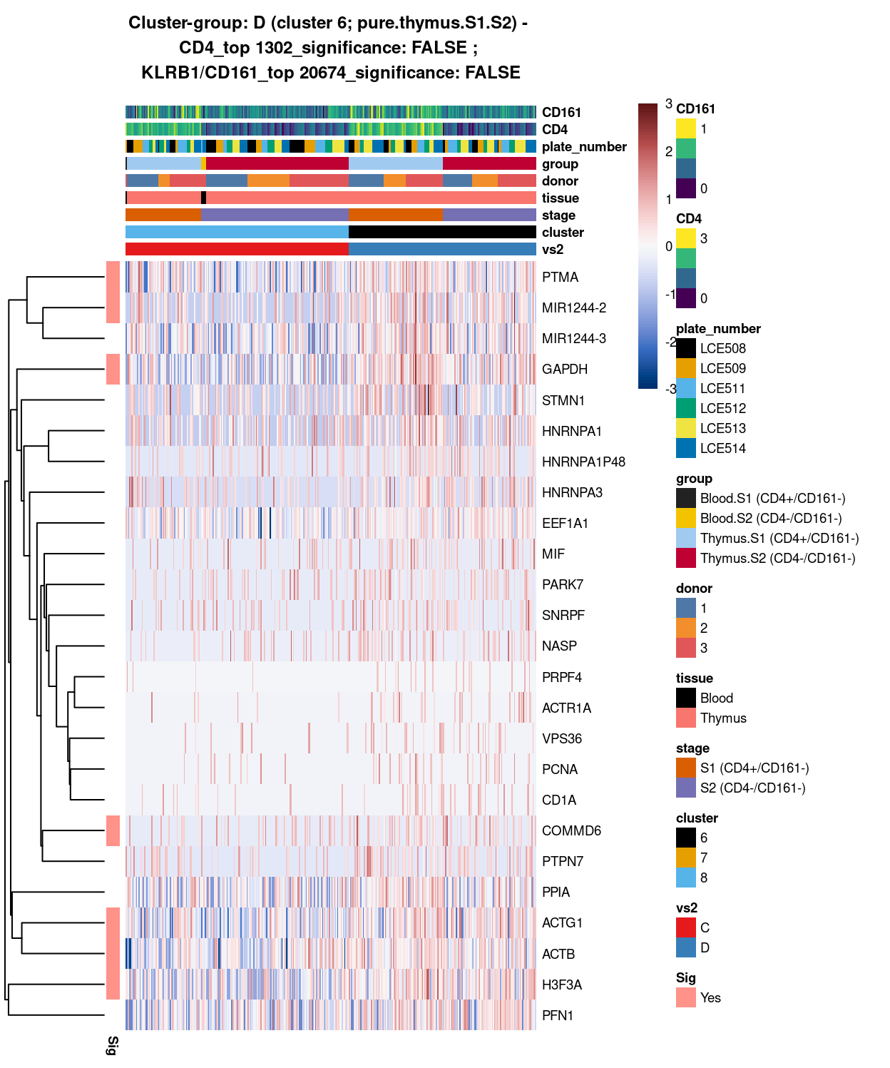
Figure 9: Heatmap of log-expression values in each sample for the top uniquely upregulated marker genes. Each column is a sample, each row a gene. Colours are capped at -3 and 3 to preserve dynamic range. Ranking of CD4 and CD161/KLRB1 from top of the DGE list sorted in ascending order of FDR and their statistical significance (TRUE = FDR < 0.05) are provided in the title.

DGE lists of these comparisons are available in output/marker_genes/S1_S2_only/uniquely_up/cluster_8_vs_6/.

SUMMARY: 8 vs 6 (C vs D)

• cluster 8 (mostly.thymus.S1.S2.less.blood >>> with markers like LTB, and the more frequently expressed DGKA, EPB41
• cluster 6 (pure.thymus.S1.S2 >>> 7 markers only, i.e. PTMA, MIR1244-2, and GAPDH, etc; maybe cluster 6 is more similar to 8, than to 7
• COMMENT: except for LTB, number of unique markers shown on either cluster, proven they are separated clusters

cluster_7_8_vs_cluster_6

Show code

#########
# E vs F
#########

##########################################################################################
# cluster 6 (i.e. pure.thymus.S1.S2) vs cluster 7_8 (i.e. mostly.thymus.S1.S2.with.blood)

# checkpoint
cp <- sce

# classify cluster-group for comparison
cp$vs3 <- factor(ifelse(cp$cluster == 6, "E", "F"))

# set vs colours
vs3_colours <- setNames(
  palette.colors(nlevels(cp$vs3), "Set1"),
  levels(cp$vs3))
cp$colours$vs3_colours <- vs3_colours[cp$vs3]

# find unique DE ./. cluster-groups
vs3_uniquely_up <- findMarkers(
  cp,
  groups = cp$vs3,
  block = cp$block,
  pval.type = "all",
  direction = "up")

# export DGE lists
saveRDS(
  vs3_uniquely_up,
  here("data", "marker_genes", "S1_S2_only", "C094_Pellicci.uniquely_up.cluster_6_vs_7_8.rds"),
  compress = "xz")

dir.create(here("output", "marker_genes", "S1_S2_only", "uniquely_up", "cluster_6_vs_7_8"), recursive = TRUE)

vs_pair <- c("6", "7_8")

message("Writing 'uniquely_up (cluster_6_vs_7_8)' marker genes to file.")
for (n in names(vs3_uniquely_up)) {
  message(n)
  gzout <- gzfile(
    description = here(
      "output",
      "marker_genes",
      "S1_S2_only",
      "uniquely_up",
      "cluster_6_vs_7_8",
      paste0("cluster_",
             vs_pair[which(names(vs3_uniquely_up) %in% n)],
             "_vs_",
             vs_pair[-which(names(vs3_uniquely_up) %in% n)][1],
             ".uniquely_up.csv.gz")),
    open = "wb")
  write.table(
    x = vs3_uniquely_up[[n]] %>%
      as.data.frame() %>%
      tibble::rownames_to_column("gene_ID"),
    file = gzout,
    sep = ",",
    quote = FALSE,
    row.names = FALSE,
    col.names = TRUE)
  close(gzout)
}

Show code

###############################################################
# look at cluster-group E / cluster 6 (i.e. pure.thymus.S1.S2)
chosen <- "E"
E_uniquely_up <- vs3_uniquely_up[[chosen]]

# add description for the chosen cluster-group
x <- "(cluster 6; pure.thymus.S1.S2)"

# look only at protein coding gene (pcg)
# NOTE: not suggest to narrow down into pcg as it remove all significant candidates (FDR << 0.05) !
# E_uniquely_up_pcg <- E_uniquely_up[intersect(protein_coding_gene_set, rownames(E_uniquely_up)), ]

# get rid of noise (i.e. pseudo, ribo, mito, sex) that collaborator not interested in
E_uniquely_up_noiseR <- E_uniquely_up[setdiff(rownames(E_uniquely_up), c(pseudogene_set, mito_set, ribo_set, sex_set)), ]

# see if key marker, "CD4 and/or ""KLRB1/CD161"", contain in the DE list + if it is "significant (i.e FDR <0.05)
y <- c("CD4",
       which(rownames(E_uniquely_up_noiseR) %in% "CD4"),
       E_uniquely_up_noiseR[which(rownames(E_uniquely_up_noiseR) %in% "CD4"), ]$FDR < 0.05)
z <- c("KLRB1/CD161",
       which(rownames(E_uniquely_up_noiseR) %in% "KLRB1"),
       E_uniquely_up_noiseR[which(rownames(E_uniquely_up_noiseR) %in% "KLRB1"), ]$FDR < 0.05)

# top25 only + gene-of-interest
best_set <- E_uniquely_up_noiseR[1:25, ]

Show code

# heatmap
plotHeatmap(
  cp,
  features = rownames(best_set),
  columns = order(
    cp$vs3,
    cp$cluster,
    cp$stage,
    cp$tissue,
    cp$donor,
    cp$group,
    cp$plate_number,
    cp$CD4,
    cp$CD161),
  colour_columns_by = c(
    "vs3",
    "cluster",
    "stage",
    "tissue",
    "donor",
    "group",
    "plate_number",
    "CD4",
    "CD161"),
  cluster_cols = FALSE,
  center = TRUE,
  symmetric = TRUE,
  zlim = c(-3, 3),
  show_colnames = FALSE,
  annotation_row = data.frame(
    Sig = factor(
      ifelse(best_set[, "FDR"] < 0.05, "Yes", "No"),
      # TODO: temp trick to deal with the row-colouring problem
      # levels = c("Yes", "No")),
      levels = c("Yes")),
    row.names = rownames(best_set)),
  main = paste0("Cluster-group: ", chosen, " ", x, " - \n",
                y[1], "_top ", y[2], "_significance: ", y[3], " ; \n",
                z[1], "_top ", z[2], "_significance: ", z[3]),
  column_annotation_colors = list(
    # Sig = c("Yes" = "red", "No" = "lightgrey"),
    vs3 = vs3_colours,
    cluster = cluster_colours,
    stage = stage_colours,
    tissue = tissue_colours,
    donor = donor_colours,
    group = group_colours,
    plate_number = plate_number_colours),
  color = hcl.colors(101, "Blue-Red 3"),
  fontsize = 7)

(#fig:heat-uniquely-up-logExp-cluster-6-vs-7_8)Heatmap of log-expression values in each sample for the top uniquely upregulated marker genes. Each column is a sample, each row a gene. Colours are capped at -3 and 3 to preserve dynamic range. Ranking of CD4 and CD161/KLRB1 from top of the DGE list sorted in ascending order of FDR and their statistical significance (TRUE = FDR < 0.05) are provided in the title.

Show code

##########################################################
# look at cluster-group F / cluster 7_8 (i.e. mostly.thymus.S1.S2.with.blood)
chosen <- "F"
F_uniquely_up <- vs3_uniquely_up[[chosen]]

# add description for the chosen cluster-group
x <- "(cluster 7_8; mostly.thymus.S1.S2.with.blood)"

# look only at protein coding gene (pcg)
# NOTE: not suggest to narrow down into pcg as it remove all significant candidates (FDR << 0.05) !
# F_uniquely_up_pcg <- F_uniquely_up[intersect(protein_coding_gene_set, rownames(F_uniquely_up)), ]

# get rid of noise (i.e. pseudo, ribo, mito, sex) that collaborator not interested in
F_uniquely_up_noiseR <- F_uniquely_up[setdiff(rownames(F_uniquely_up), c(pseudogene_set, mito_set, ribo_set, sex_set)), ]

# see if key marker, "CD4 and/or ""KLRB1/CD161"", contain in the DE list + if it is "significant (i.e FDR <0.05)
y <- c("CD4",
       which(rownames(F_uniquely_up_noiseR) %in% "CD4"),
       F_uniquely_up_noiseR[which(rownames(F_uniquely_up_noiseR) %in% "CD4"), ]$FDR < 0.05)
z <- c("KLRB1/CD161",
       which(rownames(F_uniquely_up_noiseR) %in% "KLRB1"),
       F_uniquely_up_noiseR[which(rownames(F_uniquely_up_noiseR) %in% "KLRB1"), ]$FDR < 0.05)

# top25 only + gene-of-interest
best_set <- F_uniquely_up_noiseR[1:25, ]

Show code

# heatmap
plotHeatmap(
  cp,
  features = rownames(best_set),
  columns = order(
    cp$vs3,
    cp$cluster,
    cp$stage,
    cp$tissue,
    cp$donor,
    cp$group,
    cp$plate_number,
    cp$CD4,
    cp$CD161),
  colour_columns_by = c(
    "vs3",
    "cluster",
    "stage",
    "tissue",
    "donor",
    "group",
    "plate_number",
    "CD4",
    "CD161"),
  cluster_cols = FALSE,
  center = TRUE,
  symmetric = TRUE,
  zlim = c(-3, 3),
  show_colnames = FALSE,
  annotation_row = data.frame(
    Sig = factor(
      ifelse(best_set[, "FDR"] < 0.05, "Yes", "No"),
      # TODO: temp trick to deal with the row-colouring problem
      # levels = c("Yes", "No")),
      levels = c("Yes")),
    row.names = rownames(best_set)),
  main = paste0("Cluster-group: ", chosen, " ", x, " - \n",
                y[1], "_top ", y[2], "_significance: ", y[3], " ; \n",
                z[1], "_top ", z[2], "_significance: ", z[3]),
  column_annotation_colors = list(
    # Sig = c("Yes" = "red", "No" = "lightgrey"),
    vs3 = vs3_colours,
    cluster = cluster_colours,
    stage = stage_colours,
    tissue = tissue_colours,
    donor = donor_colours,
    group = group_colours,
    plate_number = plate_number_colours),
  color = hcl.colors(101, "Blue-Red 3"),
  fontsize = 7)

(#fig:heat-uniquely-up-logExp-cluster-7_8-vs-6)Heatmap of log-expression values in each sample for the top uniquely upregulated marker genes. Each column is a sample, each row a gene. Colours are capped at -3 and 3 to preserve dynamic range. Ranking of CD4 and CD161/KLRB1 from top of the DGE list sorted in ascending order of FDR and their statistical significance (TRUE = FDR < 0.05) are provided in the title.

DGE lists of these comparisons are available in output/marker_genes/S1_S2_only/uniquely_up/cluster_6_vs_7_8/.

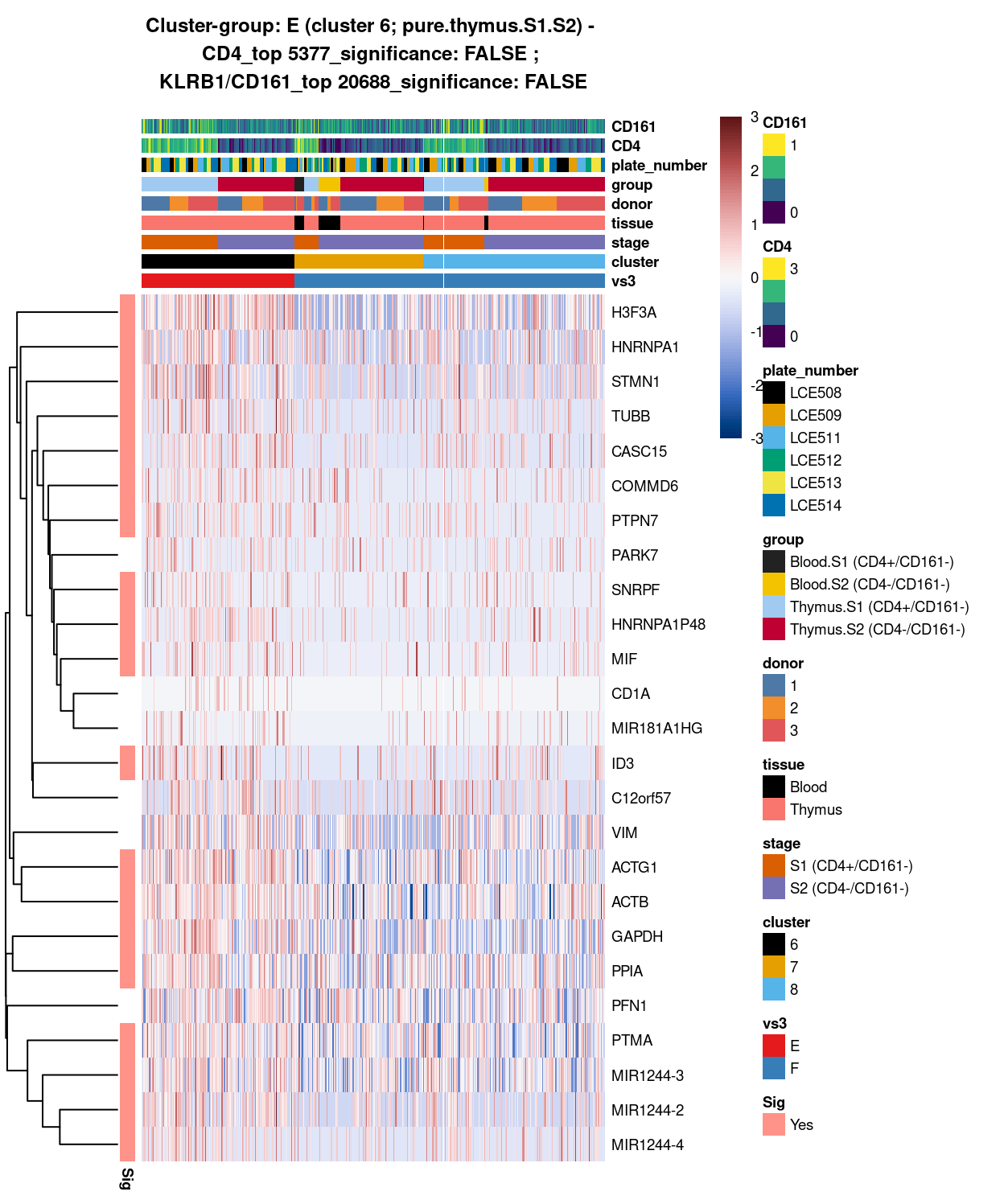
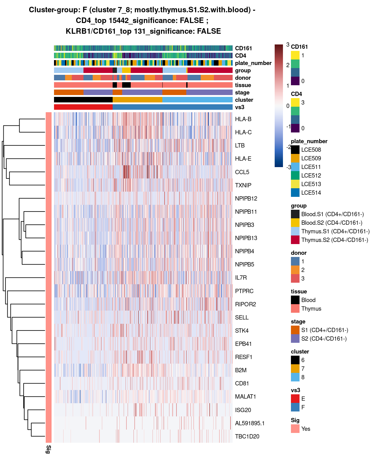
SUMMARY: 6 vs 7_8 (E vs F)

• cluster 6 (pure.thymus.S1.S2 >>> got number of markers, eg ACTG1, GAPDH, PTMA, etc
• cluster 7_8 (mostly.thymus.S1.S2.with.blood >>> also got lots of DE, eg.HLA, LTB, TXNIP; other markers like up-regulation of CCL5 and ILR7 clearly associated with cluster 2 only
• COMMENT: cluster 6 is clearly distinctive from cluster 7_8

cluster_7_vs_cluster_8

Show code

#########
# G vs H
#########

##########################################################################################
# cluster 7 (i.e. mostly.thymus.S1.S2.more.blood) vs cluster 8 (i.e. mostly.thymus.S1.S2.less.blood)

# checkpoint
cp <- sce
# exclude cells of uninterested cluster from cp
cp <- cp[, cp$cluster == "7" | cp$cluster == "8"]
colData(cp) <- droplevels(colData(cp))

# classify cluster-group for comparison
cp$vs4 <- factor(ifelse(cp$cluster == 7, "G", "H"))

# set vs colours
vs4_colours <- setNames(
  palette.colors(nlevels(cp$vs4), "Set1"),
  levels(cp$vs4))
cp$colours$vs4_colours <- vs4_colours[cp$vs4]

# find unique DE ./. cluster-groups
vs4_uniquely_up <- findMarkers(
  cp,
  groups = cp$vs4,
  block = cp$block,
  pval.type = "all",
  direction = "up")

# export DGE lists
saveRDS(
  vs4_uniquely_up,
  here("data", "marker_genes", "S1_S2_only", "C094_Pellicci.uniquely_up.cluster_7_vs_8.rds"),
  compress = "xz")

dir.create(here("output", "marker_genes", "S1_S2_only", "uniquely_up", "cluster_7_vs_8"), recursive = TRUE)

vs_pair <- c("7", "8")

message("Writing 'uniquely_up (cluster_7_vs_8)' marker genes to file.")
for (n in names(vs4_uniquely_up)) {
  message(n)
  gzout <- gzfile(
    description = here(
      "output",
      "marker_genes",
      "S1_S2_only",
      "uniquely_up",
      "cluster_7_vs_8",
      paste0("cluster_",
             vs_pair[which(names(vs4_uniquely_up) %in% n)],
             "_vs_",
             vs_pair[-which(names(vs4_uniquely_up) %in% n)][1],
             ".uniquely_up.csv.gz")),
    open = "wb")
  write.table(
    x = vs4_uniquely_up[[n]] %>%
      as.data.frame() %>%
      tibble::rownames_to_column("gene_ID"),
    file = gzout,
    sep = ",",
    quote = FALSE,
    row.names = FALSE,
    col.names = TRUE)
  close(gzout)
}

Show code

###############################################################
# look at cluster-group G / cluster 7 (i.e. mostly.thymus.S1.S2.more.blood)
chosen <- "G"
G_uniquely_up <- vs4_uniquely_up[[chosen]]

# add description for the chosen cluster-group
x <- "(cluster 7; mostly.thymus.S1.S2.more.blood)"

# look only at protein coding gene (pcg)
# NOTE: not suggest to narrow down into pcg as it remove all significant candidates (FDR << 0.05) !
# G_uniquely_up_pcg <- G_uniquely_up[intersect(protein_coding_gene_set, rownames(G_uniquely_up)), ]

# get rid of noise (i.e. pseudo, ribo, mito, sex) that collaborator not interested in
G_uniquely_up_noiseR <- G_uniquely_up[setdiff(rownames(G_uniquely_up), c(pseudogene_set, mito_set, ribo_set, sex_set)), ]

# see if key marker, "CD4 and/or ""KLRB1/CD161"", contain in the DE list + if it is "significant (i.e FDR <0.05)
y <- c("CD4",
       which(rownames(G_uniquely_up_noiseR) %in% "CD4"),
       G_uniquely_up_noiseR[which(rownames(G_uniquely_up_noiseR) %in% "CD4"), ]$FDR < 0.05)
z <- c("KLRB1/CD161",
       which(rownames(G_uniquely_up_noiseR) %in% "KLRB1"),
       G_uniquely_up_noiseR[which(rownames(G_uniquely_up_noiseR) %in% "KLRB1"), ]$FDR < 0.05)

# top25 only + gene-of-interest
best_set <- G_uniquely_up_noiseR[1:25, ]

Show code

# heatmap
plotHeatmap(
  cp,
  features = rownames(best_set),
  columns = order(
    cp$vs4,
    cp$cluster,
    cp$stage,
    cp$tissue,
    cp$donor,
    cp$group,
    cp$plate_number,
    cp$CD4,
    cp$CD161),
  colour_columns_by = c(
    "vs4",
    "cluster",
    "stage",
    "tissue",
    "donor",
    "group",
    "plate_number",
    "CD4",
    "CD161"),
  cluster_cols = FALSE,
  center = TRUE,
  symmetric = TRUE,
  zlim = c(-3, 3),
  show_colnames = FALSE,
  annotation_row = data.frame(
    Sig = factor(
      ifelse(best_set[, "FDR"] < 0.05, "Yes", "No"),
      # TODO: temp trick to deal with the row-colouring problem
      # levels = c("Yes", "No")),
      levels = c("Yes")),
    row.names = rownames(best_set)),
  main = paste0("Cluster-group: ", chosen, " ", x, " - \n",
                y[1], "_top ", y[2], "_significance: ", y[3], " ; \n",
                z[1], "_top ", z[2], "_significance: ", z[3]),
  column_annotation_colors = list(
    # Sig = c("Yes" = "red", "No" = "lightgrey"),
    vs4 = vs4_colours,
    cluster = cluster_colours,
    stage = stage_colours,
    tissue = tissue_colours,
    donor = donor_colours,
    group = group_colours,
    plate_number = plate_number_colours),
  color = hcl.colors(101, "Blue-Red 3"),
  fontsize = 7)

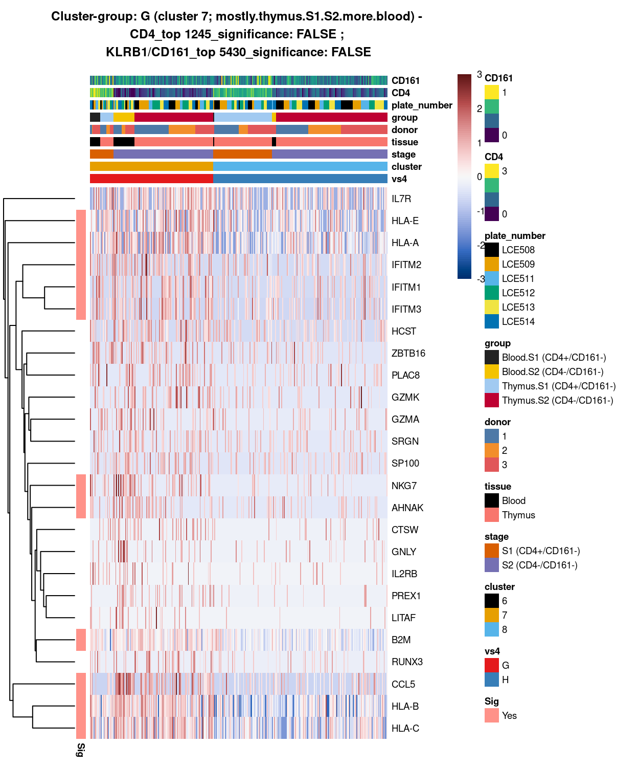
Figure 10: Heatmap of log-expression values in each sample for the top uniquely upregulated marker genes. Each column is a sample, each row a gene. Colours are capped at -3 and 3 to preserve dynamic range. Ranking of CD4 and CD161/KLRB1 from top of the DGE list sorted in ascending order of FDR and their statistical significance (TRUE = FDR < 0.05) are provided in the title.

Show code

##########################################################
# look at cluster-group H / cluster 8 (i.e. mostly.thymus.S1.S2.less.blood)
chosen <- "H"
H_uniquely_up <- vs4_uniquely_up[[chosen]]

# add description for the chosen cluster-group
x <- "(cluster 8; mostly.thymus.S1.S2.less.blood)"

# look only at protein coding gene (pcg)
# NOTE: not suggest to narrow down into pcg as it remove all significant candidates (FDR << 0.05) !
# H_uniquely_up_pcg <- H_uniquely_up[intersect(protein_coding_gene_set, rownames(H_uniquely_up)), ]

# get rid of noise (i.e. pseudo, ribo, mito, sex) that collaborator not interested in
H_uniquely_up_noiseR <- H_uniquely_up[setdiff(rownames(H_uniquely_up), c(pseudogene_set, mito_set, ribo_set, sex_set)), ]

# see if key marker, "CD4 and/or ""KLRB1/CD161"", contain in the DE list + if it is "significant (i.e FDR <0.05)
y <- c("CD4",
       which(rownames(H_uniquely_up_noiseR) %in% "CD4"),
       H_uniquely_up_noiseR[which(rownames(H_uniquely_up_noiseR) %in% "CD4"), ]$FDR < 0.05)
z <- c("KLRB1/CD161",
       which(rownames(H_uniquely_up_noiseR) %in% "KLRB1"),
       H_uniquely_up_noiseR[which(rownames(H_uniquely_up_noiseR) %in% "KLRB1"), ]$FDR < 0.05)

# top25 only + gene-of-interest
best_set <- H_uniquely_up_noiseR[1:25, ]

Show code

# heatmap
plotHeatmap(
  cp,
  features = rownames(best_set),
  columns = order(
    cp$vs4,
    cp$cluster,
    cp$stage,
    cp$tissue,
    cp$donor,
    cp$group,
    cp$plate_number,
    cp$CD4,
    cp$CD161),
  colour_columns_by = c(
    "vs4",
    "cluster",
    "stage",
    "tissue",
    "donor",
    "group",
    "plate_number",
    "CD4",
    "CD161"),
  cluster_cols = FALSE,
  center = TRUE,
  symmetric = TRUE,
  zlim = c(-3, 3),
  show_colnames = FALSE,
  annotation_row = data.frame(
    Sig = factor(
      ifelse(best_set[, "FDR"] < 0.05, "Yes", "No"),
      # TODO: temp trick to deal with the row-colouring problem
      # levels = c("Yes", "No")),
      levels = c("Yes")),
    row.names = rownames(best_set)),
  main = paste0("Cluster-group: ", chosen, " ", x, " - \n",
                y[1], "_top ", y[2], "_significance: ", y[3], " ; \n",
                z[1], "_top ", z[2], "_significance: ", z[3]),
  column_annotation_colors = list(
    # Sig = c("Yes" = "red", "No" = "lightgrey"),
    vs4 = vs4_colours,
    cluster = cluster_colours,
    stage = stage_colours,
    tissue = tissue_colours,
    donor = donor_colours,
    group = group_colours,
    plate_number = plate_number_colours),
  color = hcl.colors(101, "Blue-Red 3"),
  fontsize = 7)

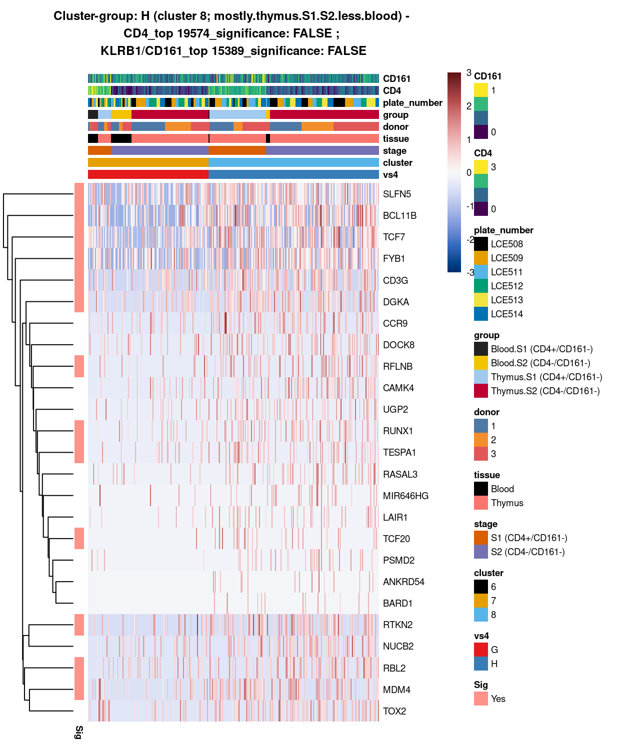
Figure 11: Heatmap of log-expression values in each sample for the top uniquely upregulated marker genes. Each column is a sample, each row a gene. Colours are capped at -3 and 3 to preserve dynamic range. Ranking of CD4 and CD161/KLRB1 from top of the DGE list sorted in ascending order of FDR and their statistical significance (TRUE = FDR < 0.05) are provided in the title.

DGE lists of these comparisons are available in output/marker_genes/S1_S2_only/uniquely_up/cluster_7_vs_8/.

SUMMARY: 7 vs 8 (E vs F)

• cluster 7 (mostly.thymus.S1.S2.more.blood >>> got number of good markers, e.g. class 1 HLA, IFITM family, NKG7, which are all more frequently expressed in cluster 7
• cluster 8 (mostly.thymus.S1.S2.less.blood >>> got another set of unique markers, eg. BCL11B, DGKA, FYB1, etc. for cluster 8
• COMMENT: there are clearly 2 distinct subtypes (though both may seem to be thymus.s1.s2 with blood, it actually indicate these sub-stages of cells with different origins share similar expression pattern !)

Selected pairwise comparisons - integrated

To have a comprehensive overview, the above analyses were summarized in the following heatmap per cluster:

Show code

# NOTE: The following is a workaround to the lack of support for tabsets in 
#       distill (see https://github.com/rstudio/distill/issues/11 and 
#       https://github.com/rstudio/distill/issues/11#issuecomment-692142414 in 
#       particular).
xaringanExtra::use_panelset()

Cluster_6_integrated

Show code

############
# cluster 6
############

chosen <- "6"
# add description for the chosen cluster-group
x <- "(pure.thymus.S1.S2)"
# retain only significant markers (FDR<0.05) + keep only required output columns
B_uniquely_up_noiseR_sig <- B_uniquely_up_noiseR[B_uniquely_up_noiseR$FDR<0.05,][ ,c(1:3)]
D_uniquely_up_noiseR_sig <- D_uniquely_up_noiseR[D_uniquely_up_noiseR$FDR<0.05,][ ,c(1:3)]
F_uniquely_up_noiseR_sig <- F_uniquely_up_noiseR[F_uniquely_up_noiseR$FDR<0.05,][ ,c(1:3)]
cluster6_uniquely_up_noiseR_sig <- cluster6_uniquely_up_noiseR[cluster6_uniquely_up_noiseR$FDR<0.05,][ ,c(1:3)]
# add top column
B_uniquely_up_noiseR_sig$top <- 1:nrow(B_uniquely_up_noiseR_sig)
D_uniquely_up_noiseR_sig$top <- 1:nrow(D_uniquely_up_noiseR_sig)
F_uniquely_up_noiseR_sig$top <- 1:nrow(F_uniquely_up_noiseR_sig)
cluster6_uniquely_up_noiseR_sig$top <- 1:nrow(cluster6_uniquely_up_noiseR_sig)
# unify S4 objects, sort by top (ascending) then FDR (ascending), keep only first unique entry for each marker
BDF6_uniquely_up_noiseR_sig <- rbind2(B_uniquely_up_noiseR_sig,
                                      D_uniquely_up_noiseR_sig,
                                      F_uniquely_up_noiseR_sig,
                                      cluster6_uniquely_up_noiseR_sig)
BDF6_uniquely_up_noiseR_sig_sort <- BDF6_uniquely_up_noiseR_sig[with(BDF6_uniquely_up_noiseR_sig, order(top, FDR)), ]
BDF6_uniquely_up_noiseR_sig_sort_uniq <- BDF6_uniquely_up_noiseR_sig_sort[unique(rownames(BDF6_uniquely_up_noiseR_sig_sort)), ]
# # de-select unannotated/ not well-characterised genes
# deselected <- c("NPIPB13", "NPIPB3", "NPIPB11", "NPIPB5", "NPIPB4", "EEF1A1", "ACTG1", "ACTB", "IFITM1")
deselected <- c("MALAT1")
BDF6_uniquely_up_noiseR_sig_sort_uniq_selected <- BDF6_uniquely_up_noiseR_sig_sort_uniq[!(rownames(BDF6_uniquely_up_noiseR_sig_sort_uniq) %in% deselected), ]

# export DGE lists
saveRDS(
  BDF6_uniquely_up_noiseR_sig_sort_uniq_selected,
  here("data", "marker_genes", "S1_S2_only", "C094_Pellicci.uniquely_up.cluster_6_integrated.rds"),
  compress = "xz")
dir.create(here("output", "marker_genes", "S1_S2_only", "uniquely_up", "integrated"), recursive = TRUE)
message("Writing 'uniquely_up (cluster_6_integrated)' marker genes to file.")
gzout <- gzfile(
  description = here(
    "output",
    "marker_genes",
    "S1_S2_only",
    "uniquely_up",
    "integrated",
    paste0("cluster_6_integrated",
           ".uniquely_up.csv.gz")),
  open = "wb")
write.table(
  x = BDF6_uniquely_up_noiseR_sig_sort_uniq_selected %>%
    as.data.frame() %>%
    tibble::rownames_to_column("gene_ID"),
  file = gzout,
  sep = ",",
  quote = FALSE,
  row.names = FALSE,
  col.names = TRUE)
close(gzout)
# top only + gene-of-interest
best_set <- BDF6_uniquely_up_noiseR_sig_sort_uniq_selected[1:50, ]

Show code

# heatmap
plotHeatmap(
  sce,
  features = rownames(best_set),
  columns = order(
    sce$cluster,
    sce$stage,
    sce$tissue,
    sce$donor,
    sce$group,
    sce$plate_number,
    sce$CD4,
    sce$CD161),
  colour_columns_by = c(
    "cluster",
    "stage",
    "tissue",
    "donor",
    "group",
    "plate_number",
    "CD4",
    "CD161"),
  cluster_cols = FALSE,
  center = TRUE,
  symmetric = TRUE,
  zlim = c(-3, 3),
  show_colnames = FALSE,
  annotation_row = data.frame(
    # TODO: temp trick to deal with the row-colouring problem
    cluster6.vs.7 = factor(ifelse(rownames(best_set) %in% rownames(B_uniquely_up_noiseR_sig), "DE", "not DE"), levels = c("DE")),
    cluster6.vs.8 = factor(ifelse(rownames(best_set) %in% rownames(D_uniquely_up_noiseR_sig), "DE", "not DE"), levels = c("DE")),
    cluster6.vs.7_8 = factor(ifelse(rownames(best_set) %in% rownames(F_uniquely_up_noiseR_sig), "DE", "not DE"), levels = c("DE")),
    cluster6.vs.7.vs.8 = factor(ifelse(rownames(best_set) %in% rownames(cluster6_uniquely_up_noiseR_sig), "DE", "not DE"), levels = c("DE")),    
    row.names = rownames(best_set)),
  main = paste0("Cluster ", chosen, " ", x),
  column_annotation_colors = list(
    # Sig = c("Yes" = "red", "No" = "lightgrey"),
    cluster = cluster_colours,
    stage = stage_colours,
    tissue = tissue_colours,
    donor = donor_colours,
    group = group_colours,
    plate_number = plate_number_colours),
  color = hcl.colors(101, "Blue-Red 3"),
  fontsize = 7)

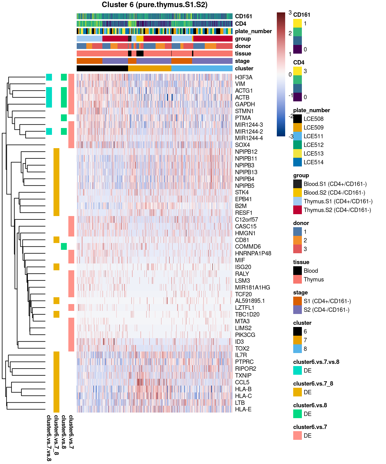
Figure 12: Heatmap of log-expression values in each sample for the top uniquely upregulated marker genes. Each column is a sample, each row a gene. Colours are capped at -3 and 3 to preserve dynamic range.

Cluster_7_integrated

Show code

############
# cluster 7
############

chosen <- "7"
# add description for the chosen cluster-group
x <- "(mostly.thymus.S1.S2.more.blood)"
# retain only significant markers (FDR<0.05) + keep only required output columns
A_uniquely_up_noiseR_sig <- A_uniquely_up_noiseR[A_uniquely_up_noiseR$FDR<0.05,][ ,c(1:3)]
G_uniquely_up_noiseR_sig <- G_uniquely_up_noiseR[G_uniquely_up_noiseR$FDR<0.05,][ ,c(1:3)]
cluster7_uniquely_up_noiseR_sig <- cluster7_uniquely_up_noiseR[cluster7_uniquely_up_noiseR$FDR<0.05,][ ,c(1:3)]
# add top column
A_uniquely_up_noiseR_sig$top <- 1:nrow(A_uniquely_up_noiseR_sig)
G_uniquely_up_noiseR_sig$top <- 1:nrow(G_uniquely_up_noiseR_sig)
cluster7_uniquely_up_noiseR_sig$top <- 1:nrow(cluster7_uniquely_up_noiseR_sig)
# unify S4 objects, sort by top (ascending) then FDR (ascending), keep only first unique entry for each marker
AG7_uniquely_up_noiseR_sig <- rbind2(A_uniquely_up_noiseR_sig,
                                     G_uniquely_up_noiseR_sig,
                                     cluster7_uniquely_up_noiseR_sig)
AG7_uniquely_up_noiseR_sig_sort <- AG7_uniquely_up_noiseR_sig[with(AG7_uniquely_up_noiseR_sig, order(top, FDR)), ]
AG7_uniquely_up_noiseR_sig_sort_uniq <- AG7_uniquely_up_noiseR_sig_sort[unique(rownames(AG7_uniquely_up_noiseR_sig_sort)), ]
# # de-select unannotated/ not well-characterised genes
# deselected <- c("NPIPB13", "NPIPB3", "NPIPB11", "NPIPB5", "NPIPB4", "EEF1A1", "ACTG1", "ACTB", "IFITM1")
deselected <- c("MALAT1")
AG7_uniquely_up_noiseR_sig_sort_uniq_selected <- AG7_uniquely_up_noiseR_sig_sort_uniq[!(rownames(AG7_uniquely_up_noiseR_sig_sort_uniq) %in% deselected), ]

# export DGE lists
saveRDS(
  AG7_uniquely_up_noiseR_sig_sort_uniq_selected,
  here("data", "marker_genes", "S1_S2_only", "C094_Pellicci.uniquely_up.cluster_7_integrated.rds"),
  compress = "xz")
dir.create(here("output", "marker_genes", "S1_S2_only", "uniquely_up", "integrated"), recursive = TRUE)
message("Writing 'uniquely_up (cluster_7_integrated)' marker genes to file.")
gzout <- gzfile(
  description = here(
    "output",
    "marker_genes",
    "S1_S2_only",
    "uniquely_up",
    "integrated",
    paste0("cluster_7_integrated",
           ".uniquely_up.csv.gz")),
  open = "wb")
write.table(
  x = AG7_uniquely_up_noiseR_sig_sort_uniq_selected %>%
    as.data.frame() %>%
    tibble::rownames_to_column("gene_ID"),
  file = gzout,
  sep = ",",
  quote = FALSE,
  row.names = FALSE,
  col.names = TRUE)
close(gzout)
# top only + gene-of-interest
# best_set <- AG7_uniquely_up_noiseR_sig_sort_uniq_selected[1:50, ]
# NOTE: only have 16 markers
best_set <- AG7_uniquely_up_noiseR_sig_sort_uniq_selected[1:16, ]

Show code

# heatmap
plotHeatmap(
  sce,
  features = rownames(best_set),
  columns = order(
    sce$cluster,
    sce$stage,
    sce$tissue,
    sce$donor,
    sce$group,
    sce$plate_number,
    sce$CD4,
    sce$CD161),
  colour_columns_by = c(
    "cluster",
    "stage",
    "tissue",
    "donor",
    "group",
    "plate_number",
    "CD4",
    "CD161"),
  cluster_cols = FALSE,
  center = TRUE,
  symmetric = TRUE,
  zlim = c(-3, 3),
  show_colnames = FALSE,
  annotation_row = data.frame(
    # TODO: temp trick to deal with the row-colouring problem
    cluster6.vs.7 = factor(ifelse(rownames(best_set) %in% rownames(A_uniquely_up_noiseR_sig), "DE", "not DE"), levels = c("DE")),
    cluster8.vs.7 = factor(ifelse(rownames(best_set) %in% rownames(G_uniquely_up_noiseR_sig), "DE", "not DE"), levels = c("DE")),
    cluster7.vs.6.vs.8 = factor(ifelse(rownames(best_set) %in% rownames(cluster7_uniquely_up_noiseR_sig), "DE", "not DE"), levels = c("DE")),    
    row.names = rownames(best_set)),
  main = paste0("Cluster ", chosen, " ", x),
  column_annotation_colors = list(
    # Sig = c("Yes" = "red", "No" = "lightgrey"),
    cluster = cluster_colours,
    stage = stage_colours,
    tissue = tissue_colours,
    donor = donor_colours,
    group = group_colours,
    plate_number = plate_number_colours),
  color = hcl.colors(101, "Blue-Red 3"),
  fontsize = 7)

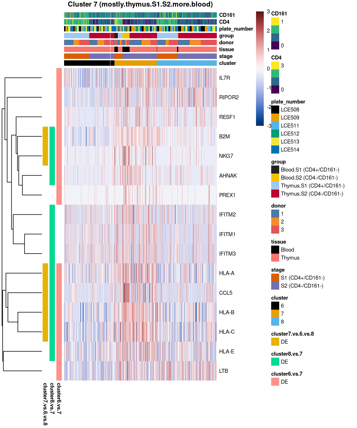
Figure 13: Heatmap of log-expression values in each sample for the top uniquely upregulated marker genes. Each column is a sample, each row a gene. Colours are capped at -3 and 3 to preserve dynamic range.

Cluster_8_integrated

Show code

############
# cluster 8
############

chosen <- "8"
# add description for the chosen cluster-group
x <- "(mostly.thymus.S1.S2.less.blood)"
# retain only significant markers (FDR<0.05) + keep only required output columns
C_uniquely_up_noiseR_sig <- C_uniquely_up_noiseR[C_uniquely_up_noiseR$FDR<0.05,][ ,c(1:3)]
H_uniquely_up_noiseR_sig <- H_uniquely_up_noiseR[H_uniquely_up_noiseR$FDR<0.05,][ ,c(1:3)]
cluster8_uniquely_up_noiseR_sig <- cluster8_uniquely_up_noiseR[cluster8_uniquely_up_noiseR$FDR<0.05,][ ,c(1:3)]
# add top column
C_uniquely_up_noiseR_sig$top <- 1:nrow(C_uniquely_up_noiseR_sig)
H_uniquely_up_noiseR_sig$top <- 1:nrow(H_uniquely_up_noiseR_sig)
# TODO: fix error - exclude list from rbind2 if empty
# cluster8_uniquely_up_noiseR_sig$top <- 1:nrow(cluster8_uniquely_up_noiseR_sig)
# unify S4 objects, sort by top (ascending) then FDR (ascending), keep only first unique entry for each marker
CH8_uniquely_up_noiseR_sig <- rbind2(C_uniquely_up_noiseR_sig,
                                     H_uniquely_up_noiseR_sig,
                                     cluster8_uniquely_up_noiseR_sig)
CH8_uniquely_up_noiseR_sig_sort <- CH8_uniquely_up_noiseR_sig[with(CH8_uniquely_up_noiseR_sig, order(top, FDR)), ]
CH8_uniquely_up_noiseR_sig_sort_uniq <- CH8_uniquely_up_noiseR_sig_sort[unique(rownames(CH8_uniquely_up_noiseR_sig_sort)), ]
# # de-select unannotated/ not well-characterised genes
# deselected <- c("NPIPB13", "NPIPB3", "NPIPB11", "NPIPB5", "NPIPB4", "EEF1A1", "ACTG1", "ACTB", "IFITM1")
deselected <- c("MALAT1")
CH8_uniquely_up_noiseR_sig_sort_uniq_selected <- CH8_uniquely_up_noiseR_sig_sort_uniq[!(rownames(CH8_uniquely_up_noiseR_sig_sort_uniq) %in% deselected), ]

# export DGE lists
saveRDS(
  CH8_uniquely_up_noiseR_sig_sort_uniq_selected,
  here("data", "marker_genes", "S1_S2_only", "C094_Pellicci.uniquely_up.cluster_8_integrated.rds"),
  compress = "xz")
dir.create(here("output", "marker_genes", "S1_S2_only", "uniquely_up", "integrated"), recursive = TRUE)
message("Writing 'uniquely_up (cluster_8_integrated)' marker genes to file.")
gzout <- gzfile(
  description = here(
    "output",
    "marker_genes",
    "S1_S2_only",
    "uniquely_up",
    "integrated",
    paste0("cluster_8_integrated",
           ".uniquely_up.csv.gz")),
  open = "wb")
write.table(
  x = CH8_uniquely_up_noiseR_sig_sort_uniq_selected %>%
    as.data.frame() %>%
    tibble::rownames_to_column("gene_ID"),
  file = gzout,
  sep = ",",
  quote = FALSE,
  row.names = FALSE,
  col.names = TRUE)
close(gzout)
# top only + gene-of-interest
# NOTE: got only 25 markers
# best_set <- CH8_uniquely_up_noiseR_sig_sort_uniq_selected[1:50, ]
best_set <- CH8_uniquely_up_noiseR_sig_sort_uniq_selected[1:25, ]

Show code

# heatmap
plotHeatmap(
  sce,
  features = rownames(best_set),
  columns = order(
    sce$cluster,
    sce$stage,
    sce$tissue,
    sce$donor,
    sce$group,
    sce$plate_number,
    sce$CD4,
    sce$CD161),
  colour_columns_by = c(
    "cluster",
    "stage",
    "tissue",
    "donor",
    "group",
    "plate_number",
    "CD4",
    "CD161"),
  cluster_cols = FALSE,
  center = TRUE,
  symmetric = TRUE,
  zlim = c(-3, 3),
  show_colnames = FALSE,
  annotation_row = data.frame(
    # TODO: temp trick to deal with the row-colouring problem
    cluster8.vs.6 = factor(ifelse(rownames(best_set) %in% rownames(C_uniquely_up_noiseR_sig), "DE", "not DE"), levels = c("DE")),
    cluster8.vs.7 = factor(ifelse(rownames(best_set) %in% rownames(H_uniquely_up_noiseR_sig), "DE", "not DE"), levels = c("DE")),
    # TODO: work out how to remove `fill` from `not_DE`
    # cluster8.vs.6.vs.7 = factor(ifelse(rownames(best_set) %in% rownames(cluster8_uniquely_up_noiseR_sig), "DE", "not DE"), levels = c("DE")),    
    row.names = rownames(best_set)),
  main = paste0("Cluster ", chosen, " ", x),
  column_annotation_colors = list(
    # Sig = c("Yes" = "red", "No" = "lightgrey"),
    cluster = cluster_colours,
    stage = stage_colours,
    tissue = tissue_colours,
    donor = donor_colours,
    group = group_colours,
    plate_number = plate_number_colours),
  color = hcl.colors(101, "Blue-Red 3"),
  fontsize = 7)

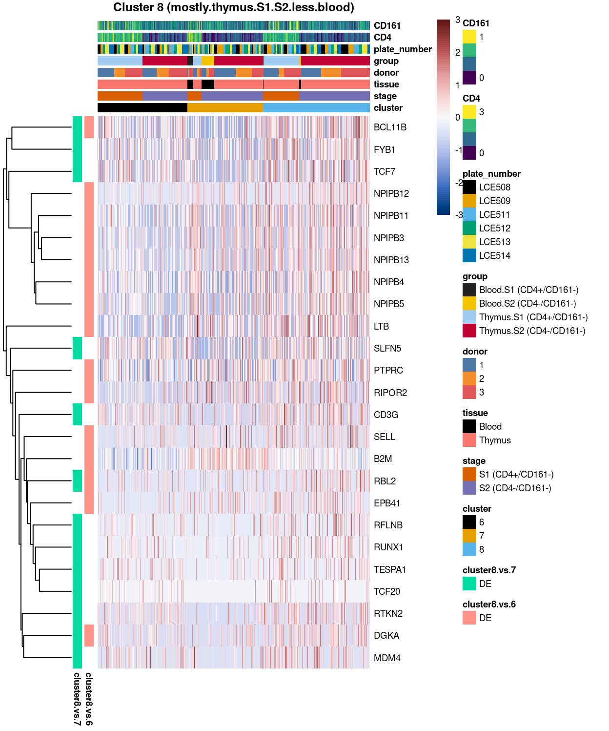
Figure 14: Heatmap of log-expression values in each sample for the top uniquely upregulated marker genes. Each column is a sample, each row a gene. Colours are capped at -3 and 3 to preserve dynamic range.

DGE lists of these comparisons are available in output/marker_genes/S1_S2_only/uniquely_up/integrated/.

Summary: Indeed, the cluster 8 (with mostly.thymus.S1.S2.less.blood) does show to have a number of genes upregulated when compared to cluster 7, such as FYB1, TCF7, CD3G etc. Whilst compared to cluster 6, cluster 8 is also featured by the statistically significant markers, such as LTB, PTPRC, and SELL, etc. Altogether, these findings indicate that there are 3 different clusters of yet-to-known cell sub-type within the S1 S2 only subset. But rather than divided by tissue (such as thymus.S1, blood.S1) or by stage (such as thymus.S1, thymus.S2), these three clusters of cell sub-types are distinguished by numbers of strong and clear up-regulation of marker genes.

Supplemental info

Comparison of key marker expression by clusters

Show code

assay(sce, "log2cpm") <- edgeR::cpm(
  counts(sce),
  log = TRUE,
  lib.size = colSums(counts(sce)))

Show code

plot_grid(
  
  # cluster 6 unique
  plotExpression(
    sce,
    features = "ACTG1",
    x = "cluster",
    exprs_values = "log2cpm",
    colour_by = "cluster") +
    theme(axis.text.x = element_text(angle = 45, hjust = 1)) +
    scale_colour_manual(values = cluster_colours, name = "cluster"),
  
  plotExpression(
    sce,
    features = "ACTB",
    x = "cluster",
    exprs_values = "log2cpm",
    colour_by = "cluster") +
    theme(axis.text.x = element_text(angle = 45, hjust = 1)) +
    scale_colour_manual(values = cluster_colours, name = "cluster"),
  
  plotExpression(
    sce,
    features = "GAPDH",
    x = "cluster",
    exprs_values = "log2cpm",
    colour_by = "cluster") +
    theme(axis.text.x = element_text(angle = 45, hjust = 1)) +
    scale_colour_manual(values = cluster_colours, name = "cluster"),
  
  plotExpression(
    sce,
    features = "MIR1244-2",
    x = "cluster",
    exprs_values = "log2cpm",
    colour_by = "cluster") +
    theme(axis.text.x = element_text(angle = 45, hjust = 1)) +
    scale_colour_manual(values = cluster_colours, name = "cluster"),

  plotExpression(
    sce,
    features = "H3F3A",
    x = "cluster",
    exprs_values = "log2cpm",
    colour_by = "cluster") +
    theme(axis.text.x = element_text(angle = 45, hjust = 1)) +
    scale_colour_manual(values = cluster_colours, name = "cluster"),
    
  # cluster 7 unique
  plotExpression(
    sce,
    features = "HLA-A",
    x = "cluster",
    exprs_values = "log2cpm",
    colour_by = "cluster") +
    theme(axis.text.x = element_text(angle = 45, hjust = 1)) +
    scale_colour_manual(values = cluster_colours, name = "cluster"),
  
  plotExpression(
    sce,
    features = "CCL5",
    x = "cluster",
    exprs_values = "log2cpm",
    colour_by = "cluster") +
    theme(axis.text.x = element_text(angle = 45, hjust = 1)) +
    scale_colour_manual(values = cluster_colours, name = "cluster"),

  plotExpression(
    sce,
    features = "NKG7",
    x = "cluster",
    exprs_values = "log2cpm",
    colour_by = "cluster") +
    theme(axis.text.x = element_text(angle = 45, hjust = 1)) +
    scale_colour_manual(values = cluster_colours, name = "cluster"),

  plotExpression(
    sce,
    features = "B2M",
    x = "cluster",
    exprs_values = "log2cpm",
    colour_by = "cluster") +
    theme(axis.text.x = element_text(angle = 45, hjust = 1)) +
    scale_colour_manual(values = cluster_colours, name = "cluster"),
  
  # cluster 8 pairwise unique (vs 7)
  plotExpression(
    sce,
    features = "FYB1",
    x = "cluster",
    exprs_values = "log2cpm",
    colour_by = "cluster") +
    theme(axis.text.x = element_text(angle = 45, hjust = 1)) +
    scale_colour_manual(values = cluster_colours, name = "cluster"),
  
  plotExpression(
    sce,
    features = "TCF7",
    x = "cluster",
    exprs_values = "log2cpm",
    colour_by = "cluster") +
    theme(axis.text.x = element_text(angle = 45, hjust = 1)) +
    scale_colour_manual(values = cluster_colours, name = "cluster"),

  plotExpression(
    sce,
    features = "CD3G",
    x = "cluster",
    exprs_values = "log2cpm",
    colour_by = "cluster") +
    theme(axis.text.x = element_text(angle = 45, hjust = 1)) +
    scale_colour_manual(values = cluster_colours, name = "cluster"),

  # cluster 8 pairwise unique (vs 6)  
  plotExpression(
    sce,
    features = "LTB",
    x = "cluster",
    exprs_values = "log2cpm",
    colour_by = "cluster") +
    theme(axis.text.x = element_text(angle = 45, hjust = 1)) +
    scale_colour_manual(values = cluster_colours, name = "cluster"),  

  plotExpression(
    sce,
    features = "PTPRC",
    x = "cluster",
    exprs_values = "log2cpm",
    colour_by = "cluster") +
    theme(axis.text.x = element_text(angle = 45, hjust = 1)) +
    scale_colour_manual(values = cluster_colours, name = "cluster"),  

  plotExpression(
    sce,
    features = "SELL",
    x = "cluster",
    exprs_values = "log2cpm",
    colour_by = "cluster") +
    theme(axis.text.x = element_text(angle = 45, hjust = 1)) +
    scale_colour_manual(values = cluster_colours, name = "cluster"),  
  
  ncol = 2)

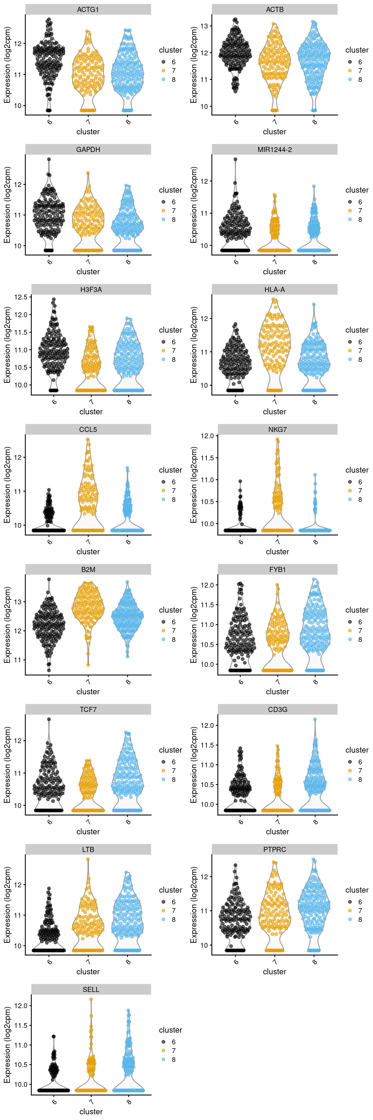
Figure 15: Violin plot showing the expression of key markers stratified by clusters

Show code

plot_grid(
  
  plotExpression(
    sce,
    features = "CCL5",
    x = "stage",
    exprs_values = "log2cpm",
    colour_by = "stage") +
    theme(axis.text.x = element_text(angle = 45, hjust = 1)) +
    scale_colour_manual(values = stage_colours, name = "stage") +
    facet_grid(~sce$tissue),   
  
  plotExpression(
    sce,
    features = "NKG7",
    x = "stage",
    exprs_values = "log2cpm",
    colour_by = "stage") +
    theme(axis.text.x = element_text(angle = 45, hjust = 1)) +
    scale_colour_manual(values = stage_colours, name = "stage") +
    facet_grid(~sce$tissue),   
  
  ncol = 1)

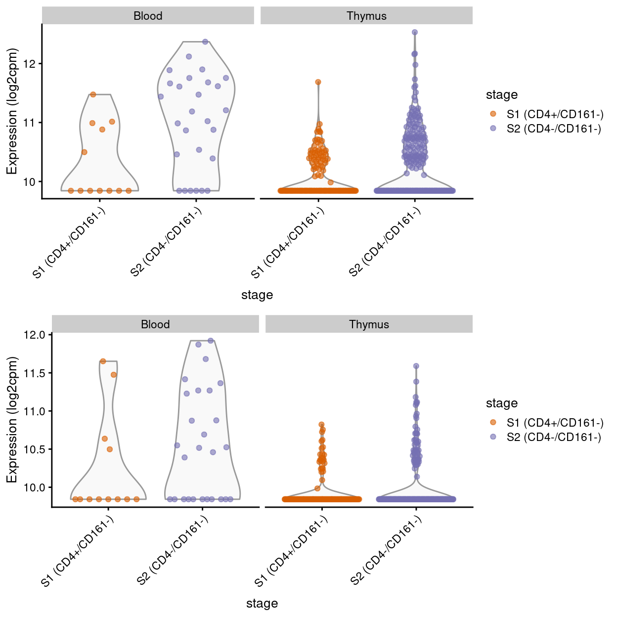
Figure 16: Violin plot showing the expression of key markers stratified by stages

Expression of minibulk DE in the single-cell dataset

Show code

###############################################
# Heatmap using minibulk sig markers as feature

# laod package for read in csv.gz
library(data.table)
library(R.utils)

# read in
a <- fread(here("output", "DEGs", "excluding_blood_1-3", "Thymus.S2_vs_Thymus.S1.aggregated_tech_reps.DEGs.csv.gz"))

# extract DEGlist (FDR < 0.05)
minibulkDEG.a <- a$ENSEMBL.GENENAME[a$FDR<0.05]

# divide the DE by UP and DOWN
minibulkDEG.a.up <- a$ENSEMBL.GENENAME[a$FDR<0.05 & a$logFC >0]
minibulkDEG.a.down <- a$ENSEMBL.GENENAME[a$FDR<0.05 & a$logFC <0]

# keep only unique markers
uniq.minibulkDEG.a <- Reduce(setdiff, list(minibulkDEG.a))
uniq.minibulkDEG.a.up <- Reduce(setdiff, list(minibulkDEG.a.up))
uniq.minibulkDEG.a.down <- Reduce(setdiff, list(minibulkDEG.a.down))

# check number of unique minibulkDEG in each
length(uniq.minibulkDEG.a)

[1] 17

Show code

length(uniq.minibulkDEG.a.up)

[1] 12

Show code

length(uniq.minibulkDEG.a.down)

[1] 5

Show code

# keep only top50
top.uniq.minibulkDEG.a <- if(length(uniq.minibulkDEG.a) >=50){uniq.minibulkDEG.a[1:50]} else {uniq.minibulkDEG.a}
minibulk_markers <- top.uniq.minibulkDEG.a

top.uniq.minibulkDEG.a.up <- if(length(uniq.minibulkDEG.a.up) >=50){uniq.minibulkDEG.a.up[1:50]} else {uniq.minibulkDEG.a.up}
minibulk_markers_up <- top.uniq.minibulkDEG.a.up

top.uniq.minibulkDEG.a.down <- if(length(uniq.minibulkDEG.a.down) >=50){uniq.minibulkDEG.a.down[1:50]} else {uniq.minibulkDEG.a.down}
minibulk_markers_down <- top.uniq.minibulkDEG.a.down

Show code

# NOTE: The following is a workaround to the lack of support for tabsets in 
#       distill (see https://github.com/rstudio/distill/issues/11 and 
#       https://github.com/rstudio/distill/issues/11#issuecomment-692142414 in 
#       particular).
xaringanExtra::use_panelset()

Minibulk DE_ALL_by cluster

Show code

library(scater)
plotHeatmap(
  sce,
  features = minibulk_markers,
  columns = order(
    sce$cluster,
    sce$stage,
    sce$tissue,
    sce$donor,
    sce$group,
    sce$plate_number),
  colour_columns_by = c(
    "cluster",
    "stage",
    "tissue",
    "donor",
    "group",
    "plate_number"),
  cluster_cols = FALSE,
  center = TRUE,
  symmetric = TRUE,
  zlim = c(-3, 3),
  show_colnames = FALSE,
  # TODO: temp trick to deal with the row-colouring problem
  annotation_row = data.frame(
    thymus.s2.vs.thymus.s1 = factor(ifelse(minibulk_markers %in% top.uniq.minibulkDEG.a, "DE", "not DE"), levels = c("DE")),
    row.names = minibulk_markers),
  main = "Minibulk DE expression (UP and DOWN) in S1 and S2 subset (with cells divided by clusters)",
  column_annotation_colors = list(
    cluster = cluster_colours,
    stage = stage_colours,
    tissue = tissue_colours,
    donor = donor_colours,
    group = group_colours,
    plate_number = plate_number_colours),
  color = hcl.colors(101, "Blue-Red 3"),
  fontsize = 7)

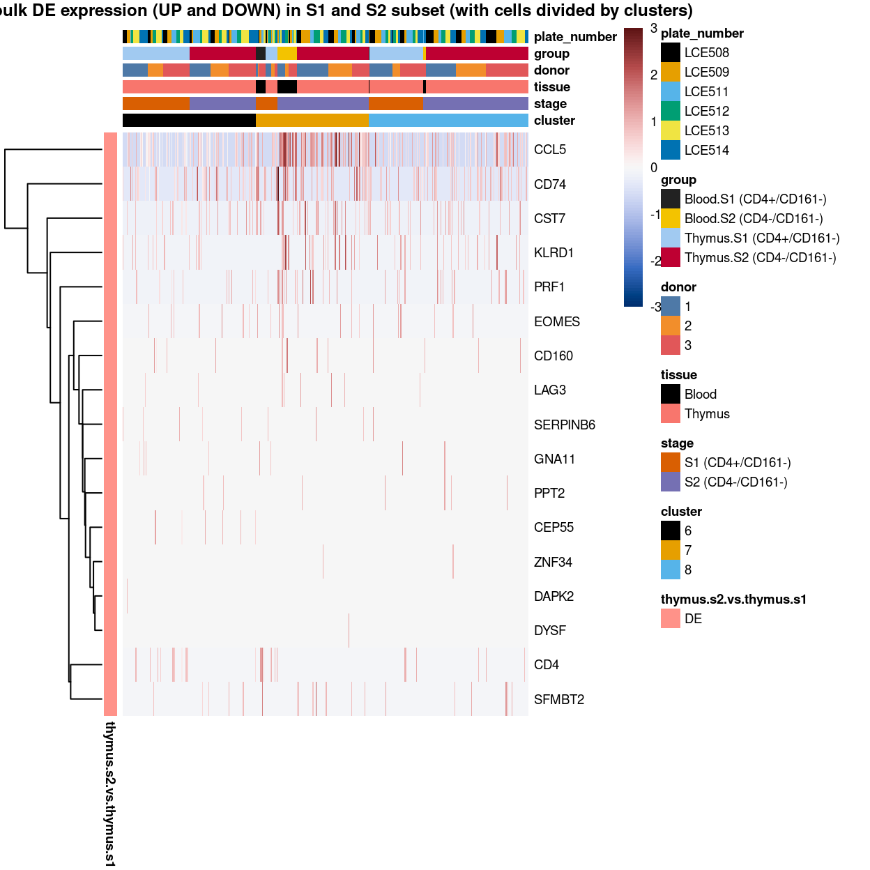
Figure 17: Heatmap of log-expression values in each sample for the marker genes identified from the mini-bulk analysis. Cells are ordered by cluster. Each column is a sample, each row a gene. Colours are capped at -3 and 3 to preserve dynamic range.

Minibulk DE_ALL_by group

Show code

library(scater)
plotHeatmap(
  sce,
  features = minibulk_markers,
  columns = order(
    sce$group,
    sce$stage,
    sce$tissue,
    sce$donor,
    sce$plate_number),
  colour_columns_by = c(
    "group",
    "stage",
    "tissue",
    "donor",
    "plate_number"),
  cluster_cols = FALSE,
  center = TRUE,
  symmetric = TRUE,
  zlim = c(-3, 3),
  show_colnames = FALSE,
  # TODO: temp trick to deal with the row-colouring problem
  annotation_row = data.frame(
    thymus.s2.vs.thymus.s1 = factor(ifelse(minibulk_markers %in% top.uniq.minibulkDEG.a, "DE", "not DE"), levels = c("DE")),
    row.names = minibulk_markers),
  main = "Minibulk DE expression (UP and DOWN) in S1 and S2 subset (with cells divided by groups)",
  column_annotation_colors = list(
    group = group_colours,
    stage = stage_colours,
    tissue = tissue_colours,
    donor = donor_colours,
    plate_number = plate_number_colours),
  color = hcl.colors(101, "Blue-Red 3"),
  fontsize = 7)

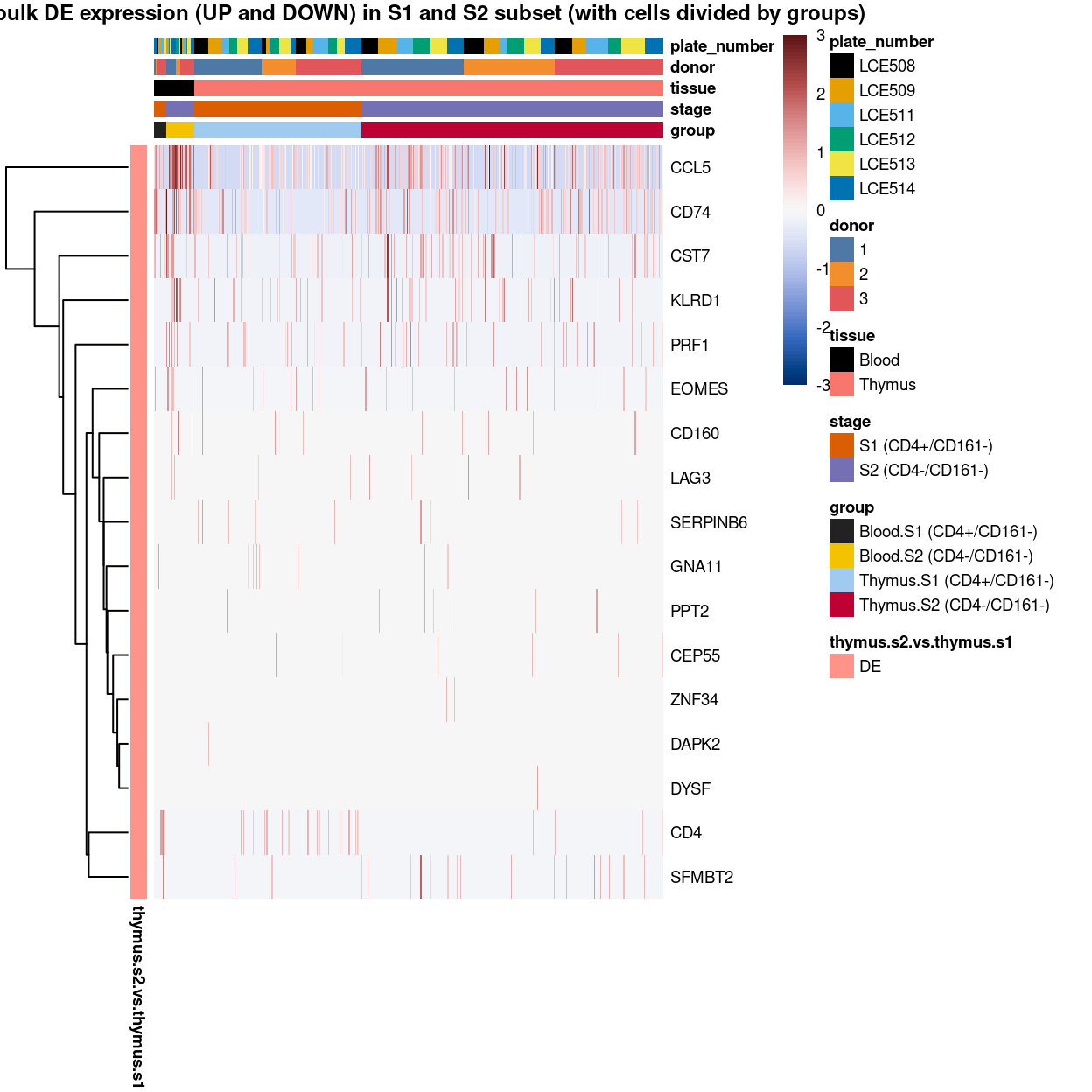
Figure 18: Heatmap of log-expression values in each sample for the marker genes identified from the mini-bulk analysis. Cells are ordered by group. Each column is a sample, each row a gene. Colours are capped at -3 and 3 to preserve dynamic range.

Minibulk DE_ALL_by group (clust_col)

Show code

library(scater)
plotHeatmap(
  sce,
  features = minibulk_markers,
  columns = order(
    sce$group,
    sce$stage,
    sce$tissue,
    sce$donor,
    sce$plate_number),
  colour_columns_by = c(
    "group",
    "stage",
    "tissue",
    "donor",
    "plate_number"),
  cluster_cols = TRUE,
  center = TRUE,
  symmetric = TRUE,
  zlim = c(-3, 3),
  show_colnames = FALSE,
  # TODO: temp trick to deal with the row-colouring problem
  annotation_row = data.frame(
    thymus.s2.vs.thymus.s1 = factor(ifelse(minibulk_markers %in% top.uniq.minibulkDEG.a, "DE", "not DE"), levels = c("DE")),
    row.names = minibulk_markers),
  main = "Minibulk DE expression (UP and DOWN) in S1 and S2 subset (with cells divided by groups, column-clustered)",
  column_annotation_colors = list(
    group = group_colours,
    stage = stage_colours,
    tissue = tissue_colours,
    donor = donor_colours,
    plate_number = plate_number_colours),
  color = hcl.colors(101, "Blue-Red 3"),
  fontsize = 7)

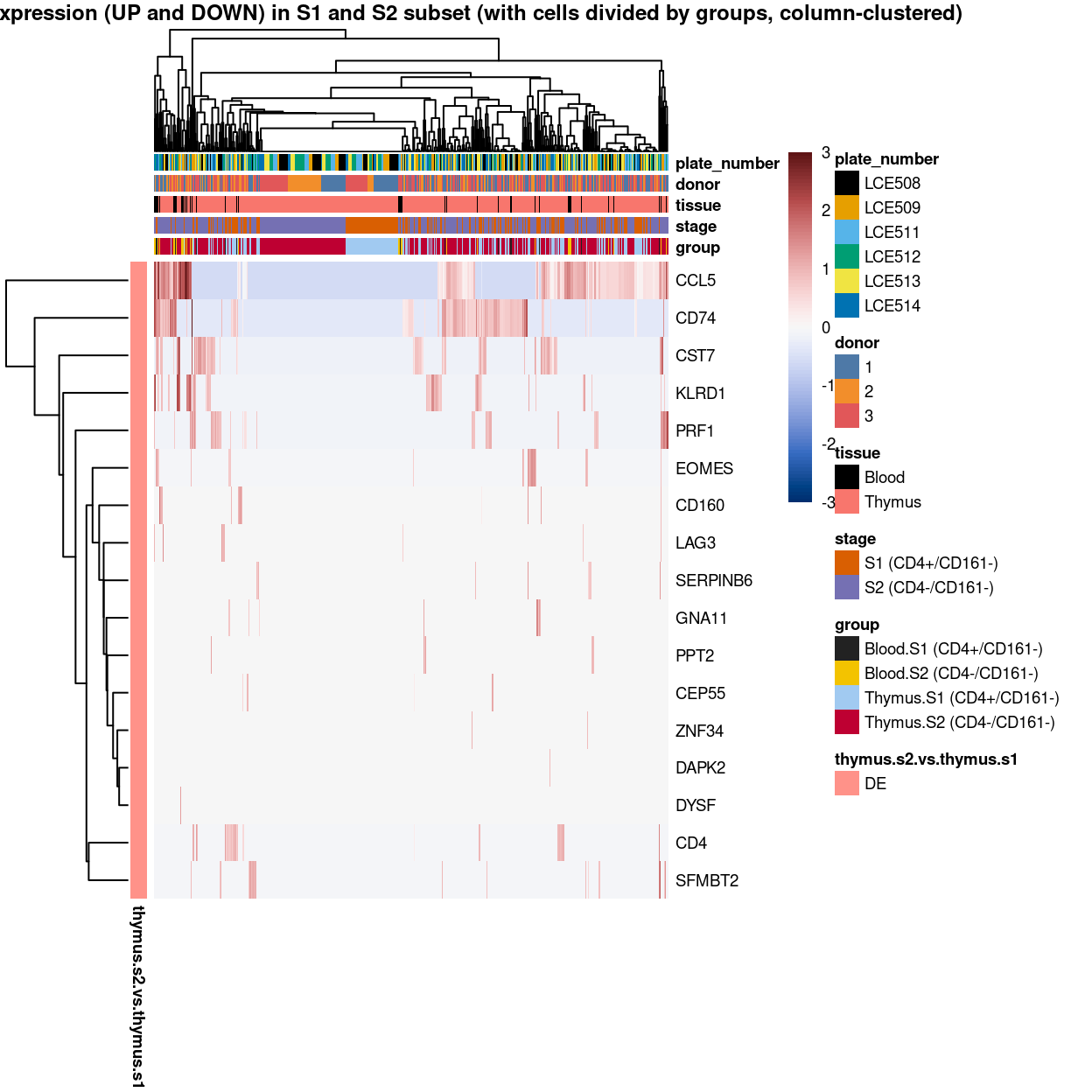
Figure 19: Heatmap of log-expression values in each sample for the marker genes identified from the mini-bulk analysis. Cells are ordered by group (column-clustered). Each column is a sample, each row a gene. Colours are capped at -3 and 3 to preserve dynamic range.

Minibulk DE_UP_by cluster

Show code

library(scater)
plotHeatmap(
  sce,
  features = minibulk_markers_up,
  columns = order(
    sce$cluster,
    sce$stage,
    sce$tissue,
    sce$donor,
    sce$group,
    sce$plate_number),
  colour_columns_by = c(
    "cluster",
    "stage",
    "tissue",
    "donor",
    "group",
    "plate_number"),
  cluster_cols = FALSE,
  center = TRUE,
  symmetric = TRUE,
  zlim = c(-3, 3),
  show_colnames = FALSE,
  # TODO: temp trick to deal with the row-colouring problem
  annotation_row = data.frame(
    thymus.s2.vs.thymus.s1 = factor(ifelse(minibulk_markers_up %in% top.uniq.minibulkDEG.a, "DE", "not DE"), levels = c("DE")),
    row.names = minibulk_markers_up),
  main = "Minibulk DE expression (UP only) in S1 and S2 subset (with cells divided by clusters)",
  column_annotation_colors = list(
    cluster = cluster_colours,
    stage = stage_colours,
    tissue = tissue_colours,
    donor = donor_colours,
    group = group_colours,
    plate_number = plate_number_colours),
  color = hcl.colors(101, "Blue-Red 3"),
  fontsize = 7)

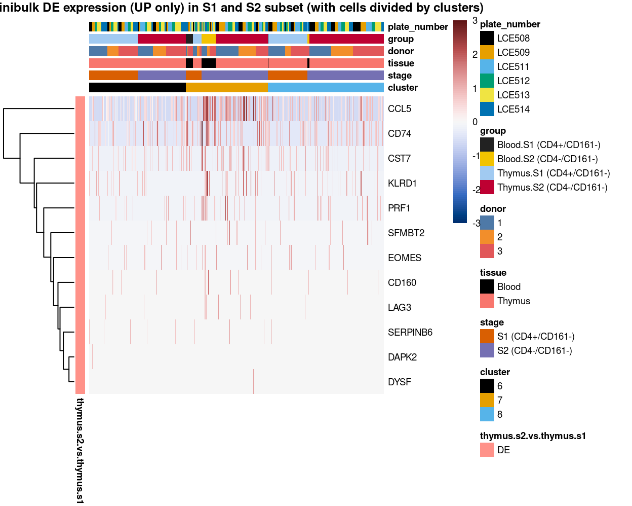
Figure 20: Heatmap of log-expression values in each sample for the marker genes (up-regulated) identified from the mini-bulk analysis. Cells are ordered by cluster. Each column is a sample, each row a gene. Colours are capped at -3 and 3 to preserve dynamic range.

Minibulk DE_UP_by group

Show code

library(scater)
plotHeatmap(
  sce,
  features = minibulk_markers_up,
  columns = order(
    sce$group,
    sce$stage,
    sce$tissue,
    sce$donor,
    sce$plate_number),
  colour_columns_by = c(
    "group",
    "stage",
    "tissue",
    "donor",
    "plate_number"),
  cluster_cols = FALSE,
  center = TRUE,
  symmetric = TRUE,
  zlim = c(-3, 3),
  show_colnames = FALSE,
  # TODO: temp trick to deal with the row-colouring problem
  annotation_row = data.frame(
    thymus.s2.vs.thymus.s1 = factor(ifelse(minibulk_markers_up %in% top.uniq.minibulkDEG.a, "DE", "not DE"), levels = c("DE")),
    row.names = minibulk_markers_up),
  main = "Minibulk DE expression (UP only) in S1 and S2 subset (with cells divided by groups)",
  column_annotation_colors = list(
    group = group_colours,
    stage = stage_colours,
    tissue = tissue_colours,
    donor = donor_colours,
    plate_number = plate_number_colours),
  color = hcl.colors(101, "Blue-Red 3"),
  fontsize = 7)

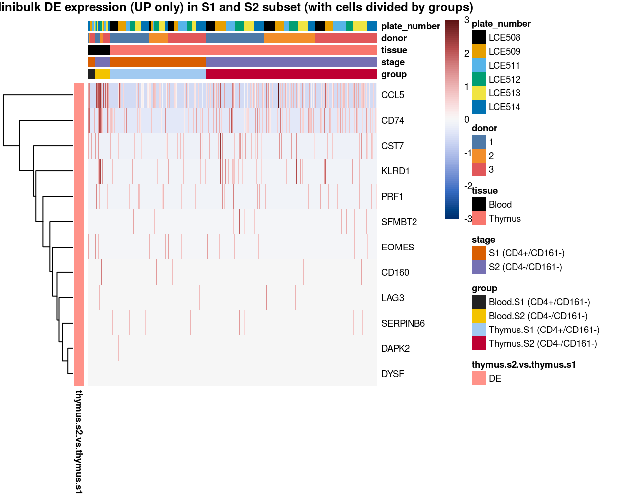
Figure 21: Heatmap of log-expression values in each sample for the marker genes (up-regulated) identified from the mini-bulk analysis. Cells are ordered by group. Each column is a sample, each row a gene. Colours are capped at -3 and 3 to preserve dynamic range.

Minibulk DE_UP_by group (clust_col)

Show code

library(scater)
plotHeatmap(
  sce,
  features = minibulk_markers_up,
  columns = order(
    sce$group,
    sce$stage,
    sce$tissue,
    sce$donor,
    sce$plate_number),
  colour_columns_by = c(
    "group",
    "stage",
    "tissue",
    "donor",
    "plate_number"),
  cluster_cols = TRUE,
  center = TRUE,
  symmetric = TRUE,
  zlim = c(-3, 3),
  show_colnames = FALSE,
  # TODO: temp trick to deal with the row-colouring problem
  annotation_row = data.frame(
    thymus.s2.vs.thymus.s1 = factor(ifelse(minibulk_markers_up %in% top.uniq.minibulkDEG.a, "DE", "not DE"), levels = c("DE")),
    row.names = minibulk_markers_up),
  main = "Minibulk DE expression (UP only) in S1 and S2 subset (with cells divided by groups, column-clustered)",
  column_annotation_colors = list(
    group = group_colours,
    stage = stage_colours,
    tissue = tissue_colours,
    donor = donor_colours,
    plate_number = plate_number_colours),
  color = hcl.colors(101, "Blue-Red 3"),
  fontsize = 7)

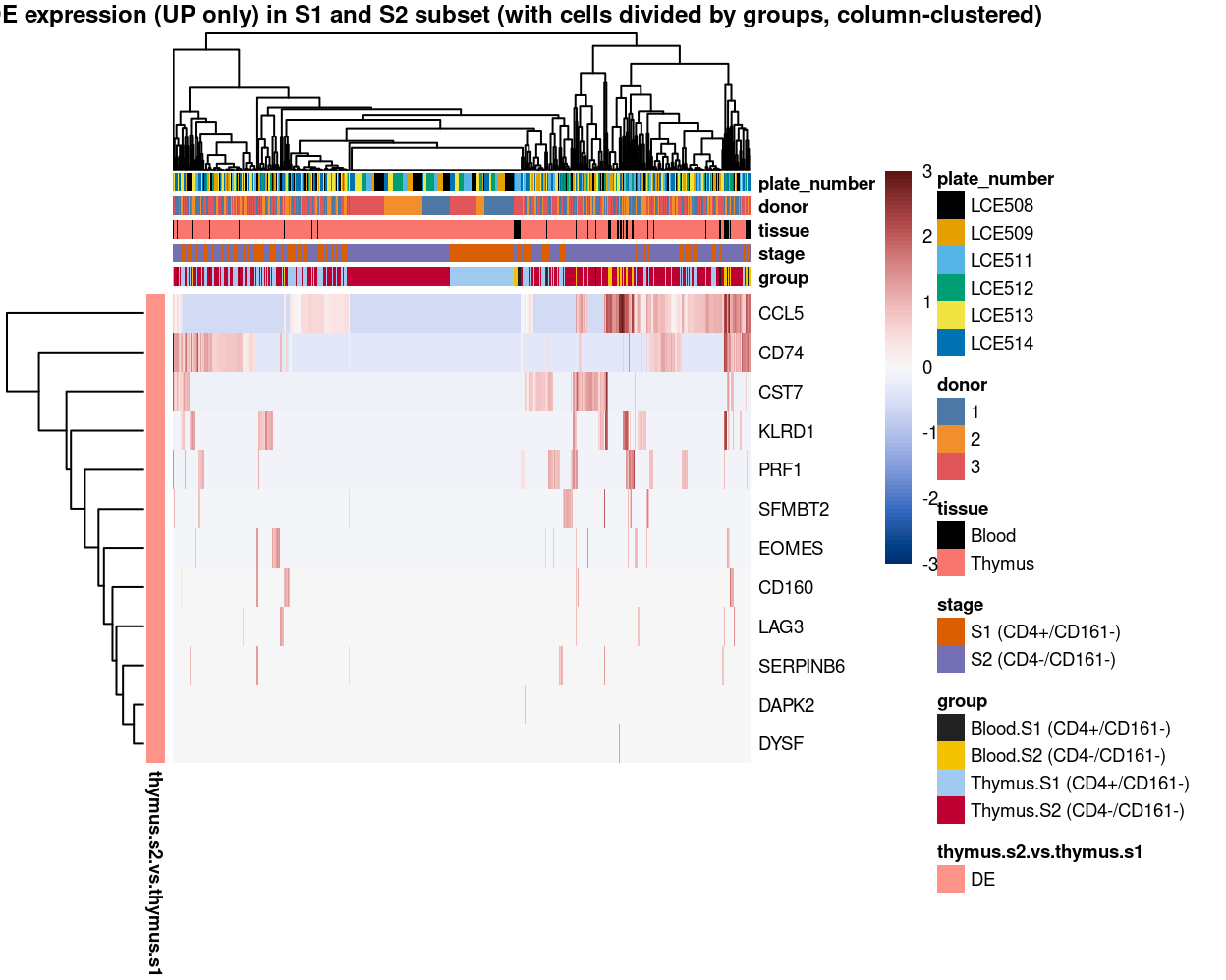
Figure 22: Heatmap of log-expression values in each sample for the marker genes (up-regulated) identified from the mini-bulk analysis. Cells are ordered by group (column-clustered). Each column is a sample, each row a gene. Colours are capped at -3 and 3 to preserve dynamic range.

Minibulk DE_DOWN_by cluster

Show code

library(scater)
plotHeatmap(
  sce,
  features = minibulk_markers_down,
  columns = order(
    sce$cluster,
    sce$stage,
    sce$tissue,
    sce$donor,
    sce$group,
    sce$plate_number),
  colour_columns_by = c(
    "cluster",
    "stage",
    "tissue",
    "donor",
    "group",
    "plate_number"),
  cluster_cols = FALSE,
  center = TRUE,
  symmetric = TRUE,
  zlim = c(-3, 3),
  show_colnames = FALSE,
  # TODO: temp trick to deal with the row-colouring problem
  annotation_row = data.frame(
    thymus.s2.vs.thymus.s1 = factor(ifelse(minibulk_markers_down %in% top.uniq.minibulkDEG.a, "DE", "not DE"), levels = c("DE")),
    row.names = minibulk_markers_down),
  main = "Minibulk DE expression (DOWN only) in S1 and S2 subset (with cells divided by clusters)",
  column_annotation_colors = list(
    cluster = cluster_colours,
    stage = stage_colours,
    tissue = tissue_colours,
    donor = donor_colours,
    group = group_colours,
    plate_number = plate_number_colours),
  color = hcl.colors(101, "Blue-Red 3"),
  fontsize = 7)

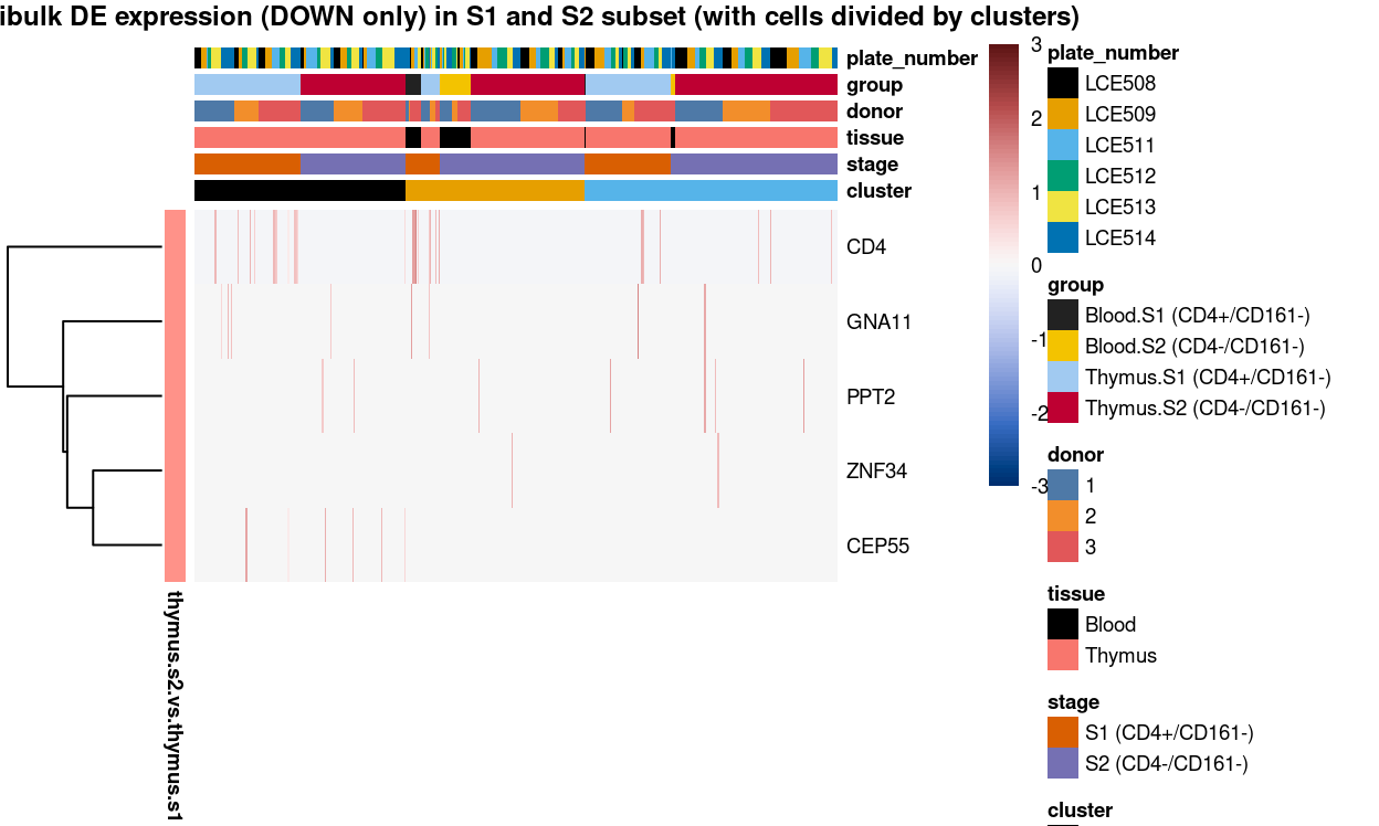
Figure 23: Heatmap of log-expression values in each sample for the marker genes (down-regulated) identified from the mini-bulk analysis. Cells are ordered by cluster. Each column is a sample, each row a gene. Colours are capped at -3 and 3 to preserve dynamic range.

Minibulk DE_DOWN_by group

Show code

library(scater)
plotHeatmap(
  sce,
  features = minibulk_markers_down,
  columns = order(
    sce$group,
    sce$stage,
    sce$tissue,
    sce$donor,
    sce$plate_number),
  colour_columns_by = c(
    "group",
    "stage",
    "tissue",
    "donor",
    "plate_number"),
  cluster_cols = FALSE,
  center = TRUE,
  symmetric = TRUE,
  zlim = c(-3, 3),
  show_colnames = FALSE,
  # TODO: temp trick to deal with the row-colouring problem
  annotation_row = data.frame(
    thymus.s2.vs.thymus.s1 = factor(ifelse(minibulk_markers_down %in% top.uniq.minibulkDEG.a, "DE", "not DE"), levels = c("DE")),
    row.names = minibulk_markers_down),
  main = "Minibulk DE expression (DOWN only) in S1 and S2 subset (with cells divided by groups)",
  column_annotation_colors = list(
    grodown = group_colours,
    stage = stage_colours,
    tissue = tissue_colours,
    donor = donor_colours,
    plate_number = plate_number_colours),
  color = hcl.colors(101, "Blue-Red 3"),
  fontsize = 7)

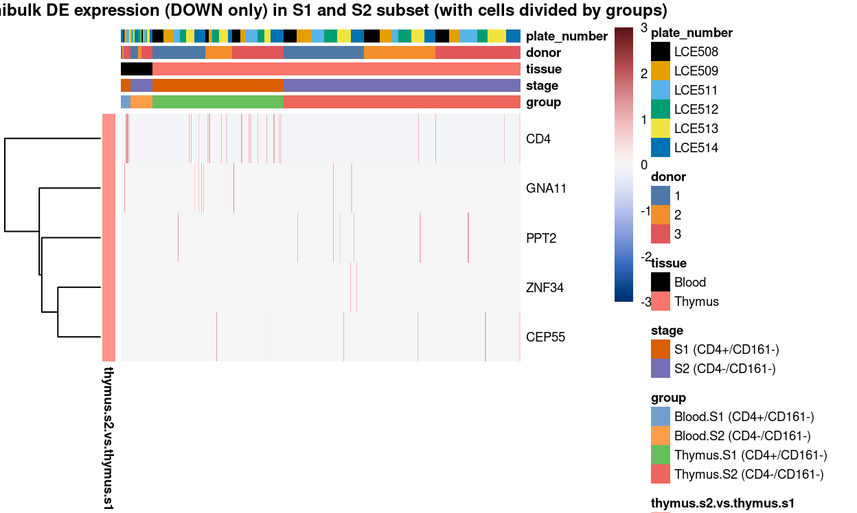
Figure 24: Heatmap of log-expression values in each sample for the marker genes (down-regulated) identified from the mini-bulk analysis. Cells are ordered by grodown. Each column is a sample, each row a gene. Colours are capped at -3 and 3 to preserve dynamic range.

Minibulk DE_DOWN_by group (clust_col)

Show code

library(scater)
plotHeatmap(
  sce,
  features = minibulk_markers_down,
  columns = order(
    sce$group,
    sce$stage,
    sce$tissue,
    sce$donor,
    sce$plate_number),
  colour_columns_by = c(
    "group",
    "stage",
    "tissue",
    "donor",
    "plate_number"),
  cluster_cols = TRUE,
  center = TRUE,
  symmetric = TRUE,
  zlim = c(-3, 3),
  show_colnames = FALSE,
  # TODO: temp trick to deal with the row-colouring problem
  annotation_row = data.frame(
    thymus.s2.vs.thymus.s1 = factor(ifelse(minibulk_markers_down %in% top.uniq.minibulkDEG.a, "DE", "not DE"), levels = c("DE")),
    row.names = minibulk_markers_down),
  main = "Minibulk DE expression (DOWN only) in S1 and S2 subset (with cells divided by groups, column-clustered)",
  column_annotation_colors = list(
    grodown = group_colours,
    stage = stage_colours,
    tissue = tissue_colours,
    donor = donor_colours,
    plate_number = plate_number_colours),
  color = hcl.colors(101, "Blue-Red 3"),
  fontsize = 7)

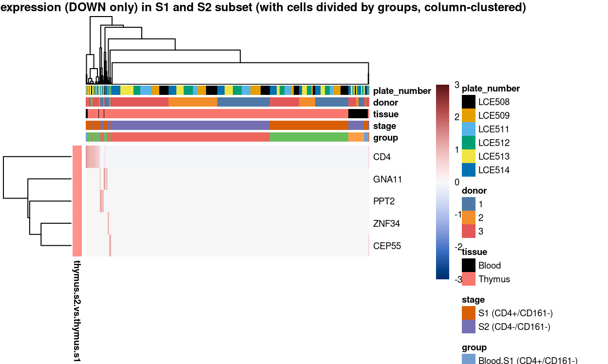
Figure 25: Heatmap of log-expression values in each sample for the marker genes (down-regulated) identified from the mini-bulk analysis. Cells are ordered by grodown (column-clustered). Each column is a sample, each row a gene. Colours are capped at -3 and 3 to preserve dynamic range.

Session info

The analysis and this document were prepared using the following software (click triangle to expand)

Show code

sessioninfo::session_info()

─ Session info ─────────────────────────────────────────────────────
 setting  value                       
 version  R version 4.0.3 (2020-10-10)
 os       CentOS Linux 7 (Core)       
 system   x86_64, linux-gnu           
 ui       X11                         
 language (EN)                        
 collate  en_US.UTF-8                 
 ctype    en_US.UTF-8                 
 tz       Australia/Melbourne         
 date     2021-09-29                  

─ Packages ─────────────────────────────────────────────────────────
 ! package              * version  date       lib
 P annotate               1.68.0   2020-10-27 [?]
 P AnnotationDbi          1.52.0   2020-10-27 [?]
 P assertthat             0.2.1    2019-03-21 [?]
 P batchelor            * 1.6.3    2021-04-16 [?]
 P beachmat               2.6.4    2020-12-20 [?]
 P beeswarm               0.3.1    2021-03-07 [?]
 P Biobase              * 2.50.0   2020-10-27 [?]
 P BiocGenerics         * 0.36.0   2020-10-27 [?]
 P BiocManager            1.30.12  2021-03-28 [?]
 P BiocNeighbors          1.8.2    2020-12-07 [?]
 P BiocParallel         * 1.24.1   2020-11-06 [?]
 P BiocSingular           1.6.0    2020-10-27 [?]
 P BiocStyle            * 2.18.1   2020-11-24 [?]
 P bit                    4.0.4    2020-08-04 [?]
 P bit64                  4.0.5    2020-08-30 [?]
 P bitops                 1.0-6    2013-08-17 [?]
 P blob                   1.2.1    2020-01-20 [?]
 P bluster                1.0.0    2020-10-27 [?]
 P bslib                  0.2.4    2021-01-25 [?]
 P cachem                 1.0.4    2021-02-13 [?]
 P cellranger             1.1.0    2016-07-27 [?]
 P cli                    2.4.0    2021-04-05 [?]
 P colorspace             2.0-0    2020-11-11 [?]
 P cowplot              * 1.1.1    2020-12-30 [?]
 P crayon                 1.4.1    2021-02-08 [?]
 P data.table           * 1.14.0   2021-02-21 [?]
 P DBI                    1.1.1    2021-01-15 [?]
 P DelayedArray           0.16.3   2021-03-24 [?]
 P DelayedMatrixStats     1.12.3   2021-02-03 [?]
 P DESeq2                 1.30.1   2021-02-19 [?]
 P digest                 0.6.27   2020-10-24 [?]
 P distill                1.2      2021-01-13 [?]
 P downlit                0.2.1    2020-11-04 [?]
 P dplyr                * 1.0.5    2021-03-05 [?]
 P dqrng                  0.2.1    2019-05-17 [?]
 P edgeR                * 3.32.1   2021-01-14 [?]
 P ellipsis               0.3.1    2020-05-15 [?]
 P evaluate               0.14     2019-05-28 [?]
 P fansi                  0.4.2    2021-01-15 [?]
 P farver                 2.1.0    2021-02-28 [?]
 P fastmap                1.1.0    2021-01-25 [?]
 P genefilter             1.72.1   2021-01-21 [?]
 P geneplotter            1.68.0   2020-10-27 [?]
 P generics               0.1.0    2020-10-31 [?]
 P GenomeInfoDb         * 1.26.4   2021-03-10 [?]
 P GenomeInfoDbData       1.2.4    2020-10-20 [?]
 P GenomicRanges        * 1.42.0   2020-10-27 [?]
 P ggbeeswarm             0.6.0    2017-08-07 [?]
 P ggplot2              * 3.3.3    2020-12-30 [?]
 P ggrepel              * 0.9.1    2021-01-15 [?]
 P Glimma               * 2.0.0    2020-10-27 [?]
 P glue                   1.4.2    2020-08-27 [?]
 P gridExtra              2.3      2017-09-09 [?]
 P gtable                 0.3.0    2019-03-25 [?]
 P here                 * 1.0.1    2020-12-13 [?]
 P highr                  0.9      2021-04-16 [?]
 P htmltools              0.5.1.1  2021-01-22 [?]
 P htmlwidgets            1.5.3    2020-12-10 [?]
 P httr                   1.4.2    2020-07-20 [?]
 P igraph                 1.2.6    2020-10-06 [?]
 P IRanges              * 2.24.1   2020-12-12 [?]
 P irlba                  2.3.3    2019-02-05 [?]
 P janitor              * 2.1.0    2021-01-05 [?]
 P jquerylib              0.1.3    2020-12-17 [?]
 P jsonlite               1.7.2    2020-12-09 [?]
 P knitr                  1.33     2021-04-24 [?]
 P labeling               0.4.2    2020-10-20 [?]
 P lattice                0.20-41  2020-04-02 [3]
 P lifecycle              1.0.0    2021-02-15 [?]
 P limma                * 3.46.0   2020-10-27 [?]
 P locfit                 1.5-9.4  2020-03-25 [?]
 P lubridate              1.7.10   2021-02-26 [?]
 P magrittr             * 2.0.1    2020-11-17 [?]
 P Matrix                 1.2-18   2019-11-27 [3]
 P MatrixGenerics       * 1.2.1    2021-01-30 [?]
 P matrixStats          * 0.58.0   2021-01-29 [?]
 P memoise                2.0.0    2021-01-26 [?]
 P msigdbr              * 7.2.1    2020-10-02 [?]
 P munsell                0.5.0    2018-06-12 [?]
 P patchwork            * 1.1.1    2020-12-17 [?]
 P pheatmap             * 1.0.12   2019-01-04 [?]
 P pillar                 1.5.1    2021-03-05 [?]
 P pkgconfig              2.0.3    2019-09-22 [?]
 P purrr                  0.3.4    2020-04-17 [?]
 P R.methodsS3          * 1.8.1    2020-08-26 [?]
 P R.oo                 * 1.24.0   2020-08-26 [?]
 P R.utils              * 2.10.1   2020-08-26 [?]
 P R6                     2.5.0    2020-10-28 [?]
 P RColorBrewer           1.1-2    2014-12-07 [?]
 P Rcpp                   1.0.6    2021-01-15 [?]
 P RCurl                  1.98-1.3 2021-03-16 [?]
 P readxl               * 1.3.1    2019-03-13 [?]
 P ResidualMatrix         1.0.0    2020-10-27 [?]
 P rlang                  0.4.11   2021-04-30 [?]
 P rmarkdown            * 2.7      2021-02-19 [?]
 P rprojroot              2.0.2    2020-11-15 [?]
 P RSQLite                2.2.5    2021-03-27 [?]
 P rsvd                   1.0.3    2020-02-17 [?]
 P S4Vectors            * 0.28.1   2020-12-09 [?]
 P sass                   0.3.1    2021-01-24 [?]
 P scales                 1.1.1    2020-05-11 [?]
 P scater               * 1.18.6   2021-02-26 [?]
 P scran                * 1.18.5   2021-02-04 [?]
 P scuttle                1.0.4    2020-12-17 [?]
 P sessioninfo            1.1.1    2018-11-05 [?]
 P SingleCellExperiment * 1.12.0   2020-10-27 [?]
 P snakecase              0.11.0   2019-05-25 [?]
 P sparseMatrixStats      1.2.1    2021-02-02 [?]
 P statmod                1.4.35   2020-10-19 [?]
 P stringi                1.7.3    2021-07-16 [?]
 P stringr                1.4.0    2019-02-10 [?]
 P SummarizedExperiment * 1.20.0   2020-10-27 [?]
 P survival               3.2-7    2020-09-28 [3]
 P tibble                 3.1.0    2021-02-25 [?]
 P tidyr                * 1.1.3    2021-03-03 [?]
 P tidyselect             1.1.0    2020-05-11 [?]
 P utf8                   1.2.1    2021-03-12 [?]
 P vctrs                  0.3.7    2021-03-29 [?]
 P vipor                  0.4.5    2017-03-22 [?]
 P viridis                0.5.1    2018-03-29 [?]
 P viridisLite            0.3.0    2018-02-01 [?]
 P withr                  2.4.1    2021-01-26 [?]
 P xaringanExtra          0.5.4    2021-08-04 [?]
 P xfun                   0.24     2021-06-15 [?]
 P XML                    3.99-0.6 2021-03-16 [?]
 P xtable                 1.8-4    2019-04-21 [?]
 P XVector                0.30.0   2020-10-27 [?]
 P yaml                   2.2.1    2020-02-01 [?]
 P zlibbioc               1.36.0   2020-10-27 [?]
 source                                  
 Bioconductor                            
 Bioconductor                            
 CRAN (R 4.0.0)                          
 Bioconductor                            
 Bioconductor                            
 CRAN (R 4.0.3)                          
 Bioconductor                            
 Bioconductor                            
 CRAN (R 4.0.3)                          
 Bioconductor                            
 Bioconductor                            
 Bioconductor                            
 Bioconductor                            
 CRAN (R 4.0.0)                          
 CRAN (R 4.0.0)                          
 CRAN (R 4.0.0)                          
 CRAN (R 4.0.0)                          
 Bioconductor                            
 CRAN (R 4.0.3)                          
 CRAN (R 4.0.3)                          
 CRAN (R 4.0.0)                          
 CRAN (R 4.0.3)                          
 CRAN (R 4.0.3)                          
 CRAN (R 4.0.3)                          
 CRAN (R 4.0.3)                          
 CRAN (R 4.0.3)                          
 CRAN (R 4.0.3)                          
 Bioconductor                            
 Bioconductor                            
 Bioconductor                            
 CRAN (R 4.0.2)                          
 CRAN (R 4.0.3)                          
 CRAN (R 4.0.3)                          
 CRAN (R 4.0.3)                          
 CRAN (R 4.0.0)                          
 Bioconductor                            
 CRAN (R 4.0.0)                          
 CRAN (R 4.0.0)                          
 CRAN (R 4.0.3)                          
 CRAN (R 4.0.3)                          
 CRAN (R 4.0.3)                          
 Bioconductor                            
 Bioconductor                            
 CRAN (R 4.0.3)                          
 Bioconductor                            
 Bioconductor                            
 Bioconductor                            
 CRAN (R 4.0.0)                          
 CRAN (R 4.0.3)                          
 CRAN (R 4.0.3)                          
 Bioconductor                            
 CRAN (R 4.0.0)                          
 CRAN (R 4.0.0)                          
 CRAN (R 4.0.0)                          
 CRAN (R 4.0.3)                          
 CRAN (R 4.0.3)                          
 CRAN (R 4.0.3)                          
 CRAN (R 4.0.3)                          
 CRAN (R 4.0.0)                          
 CRAN (R 4.0.2)                          
 Bioconductor                            
 CRAN (R 4.0.0)                          
 CRAN (R 4.0.3)                          
 CRAN (R 4.0.3)                          
 CRAN (R 4.0.3)                          
 CRAN (R 4.0.3)                          
 CRAN (R 4.0.0)                          
 CRAN (R 4.0.3)                          
 CRAN (R 4.0.3)                          
 Bioconductor                            
 CRAN (R 4.0.0)                          
 CRAN (R 4.0.3)                          
 CRAN (R 4.0.3)                          
 CRAN (R 4.0.3)                          
 Bioconductor                            
 CRAN (R 4.0.3)                          
 CRAN (R 4.0.3)                          
 CRAN (R 4.0.2)                          
 CRAN (R 4.0.0)                          
 CRAN (R 4.0.3)                          
 CRAN (R 4.0.0)                          
 CRAN (R 4.0.3)                          
 CRAN (R 4.0.0)                          
 CRAN (R 4.0.0)                          
 CRAN (R 4.0.0)                          
 CRAN (R 4.0.0)                          
 CRAN (R 4.0.0)                          
 CRAN (R 4.0.2)                          
 CRAN (R 4.0.0)                          
 CRAN (R 4.0.3)                          
 CRAN (R 4.0.3)                          
 CRAN (R 4.0.0)                          
 Bioconductor                            
 CRAN (R 4.0.5)                          
 CRAN (R 4.0.3)                          
 CRAN (R 4.0.3)                          
 CRAN (R 4.0.3)                          
 CRAN (R 4.0.0)                          
 Bioconductor                            
 CRAN (R 4.0.3)                          
 CRAN (R 4.0.0)                          
 Bioconductor                            
 Bioconductor                            
 Bioconductor                            
 CRAN (R 4.0.0)                          
 Bioconductor                            
 CRAN (R 4.0.0)                          
 Bioconductor                            
 CRAN (R 4.0.2)                          
 CRAN (R 4.0.3)                          
 CRAN (R 4.0.0)                          
 Bioconductor                            
 CRAN (R 4.0.3)                          
 CRAN (R 4.0.3)                          
 CRAN (R 4.0.3)                          
 CRAN (R 4.0.0)                          
 CRAN (R 4.0.3)                          
 CRAN (R 4.0.3)                          
 CRAN (R 4.0.0)                          
 CRAN (R 4.0.0)                          
 CRAN (R 4.0.0)                          
 CRAN (R 4.0.3)                          
 Github (gadenbuie/xaringanExtra@5e2d80b)
 CRAN (R 4.0.3)                          
 CRAN (R 4.0.3)                          
 CRAN (R 4.0.0)                          
 Bioconductor                            
 CRAN (R 4.0.0)                          
 Bioconductor                            

[1] /stornext/Projects/score/Analyses/C094_Pellicci/renv/library/R-4.0/x86_64-pc-linux-gnu
[2] /tmp/RtmpP41dVI/renv-system-library
[3] /stornext/System/data/apps/R/R-4.0.3/lib64/R/library

 P ── Loaded and on-disk path mismatch.

---

1. Differential expression analyses is performed on the original log-expression values. We do not use the MNN-corrected values here except to obtain the clusters to be characterized.↩︎