Annotating Pellicci gamma-delta T-cell single-cell dataset (S3 only)

Show code

library(SingleCellExperiment)
library(here)
library(scater)
library(scran)
library(ggplot2)
library(cowplot)
library(edgeR)
library(Glimma)
library(BiocParallel)
library(patchwork)
library(janitor)
library(pheatmap)
library(batchelor)
library(rmarkdown)
library(BiocStyle)
library(readxl)
library(dplyr)
library(tidyr)
library(ggrepel)
library(magrittr)

knitr::opts_chunk$set(fig.path = "C094_Pellicci.single-cell.annotate.S3_only_files/")

Preparing the data

We start from the cell selected SingleCellExperiment object created in ‘Merging cells for Pellicci gamma-delta T-cell dataset (S3 only)’.

Show code

sce <- readRDS(here("data", "SCEs", "C094_Pellicci.single-cell.merged.S3_only.SCE.rds"))

# pre-create directories for saving export, or error (dir not exists)
dir.create(here("data", "marker_genes", "S3_only"), recursive = TRUE)
dir.create(here("output", "marker_genes", "S3_only"), recursive = TRUE)

# Some useful colours
plate_number_colours <- setNames(
  unique(sce$colours$plate_number_colours),
  unique(names(sce$colours$plate_number_colours)))
plate_number_colours <- plate_number_colours[levels(sce$plate_number)]
tissue_colours <- setNames(
  unique(sce$colours$tissue_colours),
  unique(names(sce$colours$tissue_colours)))
tissue_colours <- tissue_colours[levels(sce$tissue)]
donor_colours <- setNames(
  unique(sce$colours$donor_colours),
  unique(names(sce$colours$donor_colours)))
donor_colours <- donor_colours[levels(sce$donor)]
stage_colours <- setNames(
  unique(sce$colours$stage_colours),
  unique(names(sce$colours$stage_colours)))
stage_colours <- stage_colours[levels(sce$stage)]
group_colours <- setNames(
  unique(sce$colours$group_colours),
  unique(names(sce$colours$group_colours)))
group_colours <- group_colours[levels(sce$group)]
cluster_colours <- setNames(
  unique(sce$colours$cluster_colours),
  unique(names(sce$colours$cluster_colours)))
cluster_colours <- cluster_colours[levels(sce$cluster)]

# Some useful gene sets
mito_set <- rownames(sce)[any(rowData(sce)$ENSEMBL.SEQNAME == "MT")]
ribo_set <- grep("^RP(S|L)", rownames(sce), value = TRUE)
# NOTE: A more curated approach for identifying ribosomal protein genes
#       (https://github.com/Bioconductor/OrchestratingSingleCellAnalysis-base/blob/ae201bf26e3e4fa82d9165d8abf4f4dc4b8e5a68/feature-selection.Rmd#L376-L380)
library(msigdbr)
c2_sets <- msigdbr(species = "Homo sapiens", category = "C2")
ribo_set <- union(
  ribo_set,
  c2_sets[c2_sets$gs_name == "KEGG_RIBOSOME", ]$gene_symbol)
ribo_set <- intersect(ribo_set, rownames(sce))
sex_set <- rownames(sce)[any(rowData(sce)$ENSEMBL.SEQNAME %in% c("X", "Y"))]
pseudogene_set <- rownames(sce)[
  any(grepl("pseudogene", rowData(sce)$ENSEMBL.GENEBIOTYPE))]
# NOTE: not suggest to narrow down into protein coding genes (pcg) as it remove all significant candidate in most of the comparison !!!
protein_coding_gene_set <- rownames(sce)[
  any(grepl("protein_coding", rowData(sce)$ENSEMBL.GENEBIOTYPE))]

Show code

# include part of the FACS data (for plot of heatmap)
facs <- t(assays(altExp(sce, "FACS"))$pseudolog)
facs_markers <- grep("V525_50_A_CD4_BV510|B530_30_A_CD161_FITC", colnames(facs), value = TRUE)
facs_selected <- facs[,facs_markers]
colnames(facs_selected) <- c("CD161", "CD4")
colData(sce) <- cbind(colData(sce), facs_selected)

Re-clustering

NOTE: Based on our explorative data analyses (EDA) on the S3 only subset, we conclude the optimal number of clusters for demonstrating the heterogeneity of the dataset, we therefore re-cluster in here. Also, as indicated by Dan during our online meeting on 11 Aug 2011, we need to use different numbering and colouring for clusters in different subsets of the dataset (to prepare for publication), we perform all these by the following script.

Show code

# re-clustering
set.seed(4759)
snn_gr <- buildSNNGraph(sce, use.dimred = "corrected", k=20)
clusters <- igraph::cluster_louvain(snn_gr)
sce$cluster <- factor(clusters$membership)

# re-numbering of clusters
sce$cluster <- factor(
  dplyr::case_when(
    sce$cluster == "1" ~ "9",
    sce$cluster == "2" ~ "10",
    sce$cluster == "3" ~ "11",
    sce$cluster == "4" ~ "12"), levels = c("9", "10", "11", "12"))

# re-colouring of clusters
cluster_colours <- setNames(
  palette.colors(nlevels(sce$cluster), "Tableau"),
  levels(sce$cluster))

After the re-clustering, there are 4 clusters for S3 only subset of the dataset.

Data overview

Show code

p1 <- plotReducedDim(sce, "UMAP_corrected", colour_by = "cluster", theme_size = 7, point_size = 0.4) +
  scale_colour_manual(values = cluster_colours, name = "cluster")
p2 <- plotReducedDim(sce, "UMAP_corrected", colour_by = "stage", theme_size = 7, point_size = 0.4) +
  scale_colour_manual(values = stage_colours, name = "stage")
p3 <- plotReducedDim(sce, "UMAP_corrected", colour_by = "plate_number", theme_size = 7, point_size = 0.4) +
  scale_colour_manual(values = plate_number_colours, name = "plate_number")
p4 <- plotReducedDim(sce, "UMAP_corrected", colour_by = "tissue", theme_size = 7, point_size = 0.4) +
  scale_colour_manual(values = tissue_colours, name = "tissue")
p5 <- plotReducedDim(sce, "UMAP_corrected", colour_by = "donor", theme_size = 7, point_size = 0.4) +
  scale_colour_manual(values = donor_colours, name = "donor")
p6 <- plotReducedDim(sce, "UMAP_corrected", colour_by = "group", theme_size = 7, point_size = 0.4) +
  scale_colour_manual(values = group_colours, name = "group")
(p1 | p2) / (p3 | p4) / (p5 | p6)

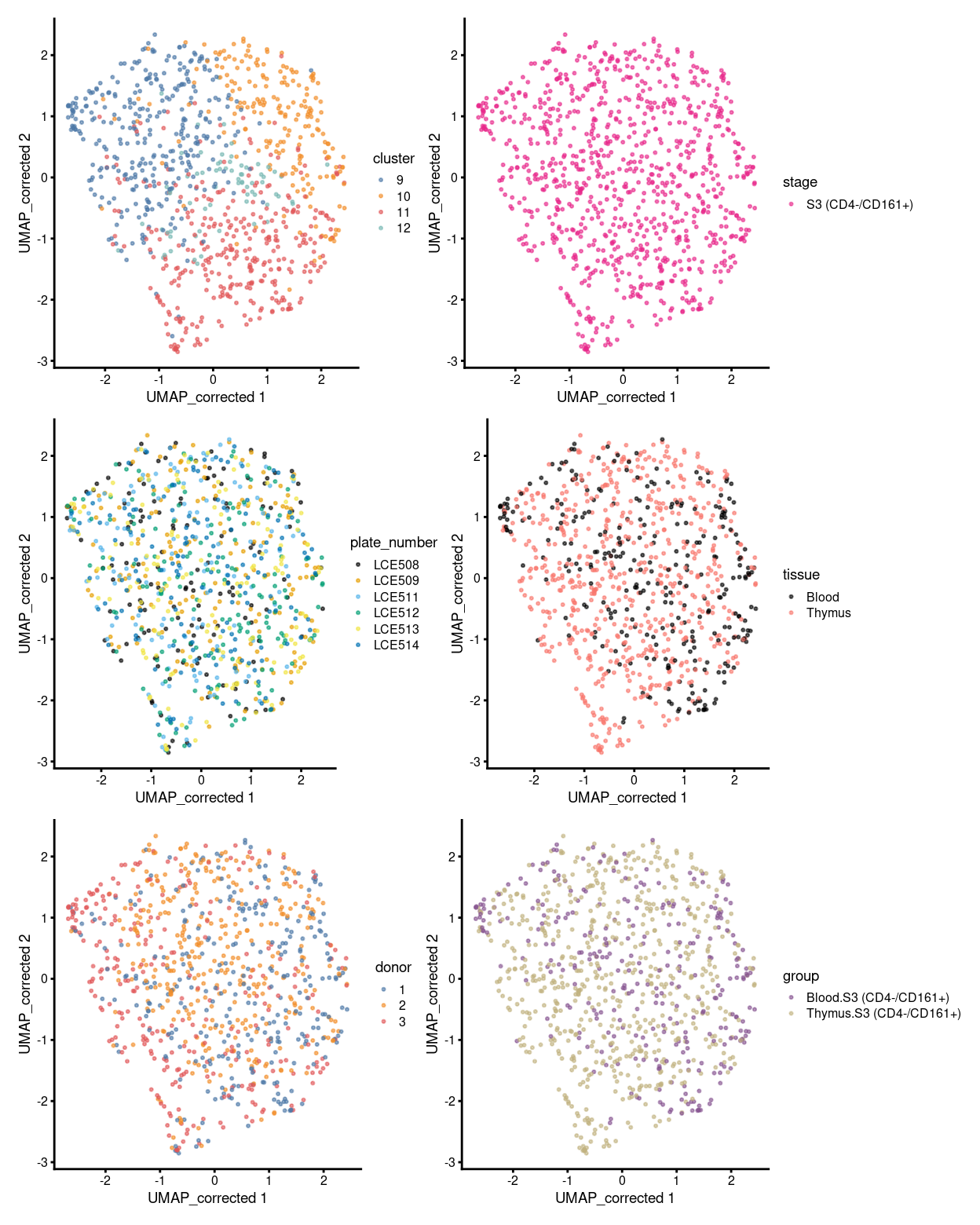
Figure 1: UMAP plot, where each point represents a cell and is coloured according to the legend.

PDF version of this figure is available in output/figures/clusterplot-umap.single-cell.annotate.S3_only.pdf.

Show code

# NOTE: A potential figure for supplementary material.
pdf(
  here("output/figures/clusterplot-umap.single-cell.annotate.S3_only.pdf"),
  height = 7.5, 
  width = 6)
(p1 | p2) / (p3 | p4) / (p5 | p6)
dev.off()

png 
  2 

Show code

dev.off()

null device 
          1 

Show code

# summary - stacked barplot
p1 <- ggcells(sce) +
  geom_bar(aes(x = cluster, fill = cluster)) +
  coord_flip() +
  ylab("Number of samples") +
  theme_cowplot(font_size = 8) +
  scale_fill_manual(values = cluster_colours) +
  geom_text(stat='count', aes(x = cluster, label=..count..), hjust=1.5, size=2)
p2 <- ggcells(sce) +
  geom_bar(
    aes(x = cluster, fill = stage),
    position = position_fill(reverse = TRUE)) +
  coord_flip() +
  ylab("Frequency") +
  scale_fill_manual(values = stage_colours) +
  theme_cowplot(font_size = 8)
p3 <- ggcells(sce) +
  geom_bar(
    aes(x = cluster, fill = plate_number),
    position = position_fill(reverse = TRUE)) +
  coord_flip() +
  ylab("Frequency") +
  scale_fill_manual(values = plate_number_colours) +
  theme_cowplot(font_size = 8)
p4 <- ggcells(sce) +
  geom_bar(
    aes(x = cluster, fill = tissue),
    position = position_fill(reverse = TRUE)) +
  coord_flip() +
  ylab("Frequency") +
  scale_fill_manual(values = tissue_colours) +
  theme_cowplot(font_size = 8)
p5 <- ggcells(sce) +
  geom_bar(
    aes(x = cluster, fill = donor),
    position = position_fill(reverse = TRUE)) +
  coord_flip() +
  ylab("Frequency") +
  scale_fill_manual(values = donor_colours) +
  theme_cowplot(font_size = 8)
p6 <- ggcells(sce) +
  geom_bar(
    aes(x = cluster, fill = group),
    position = position_fill(reverse = TRUE)) +
  coord_flip() +
  ylab("Frequency") +
  scale_fill_manual(values = group_colours) +
  theme_cowplot(font_size = 8)
(p1 | p2) / (p3 | p4) / (p5 | p6)

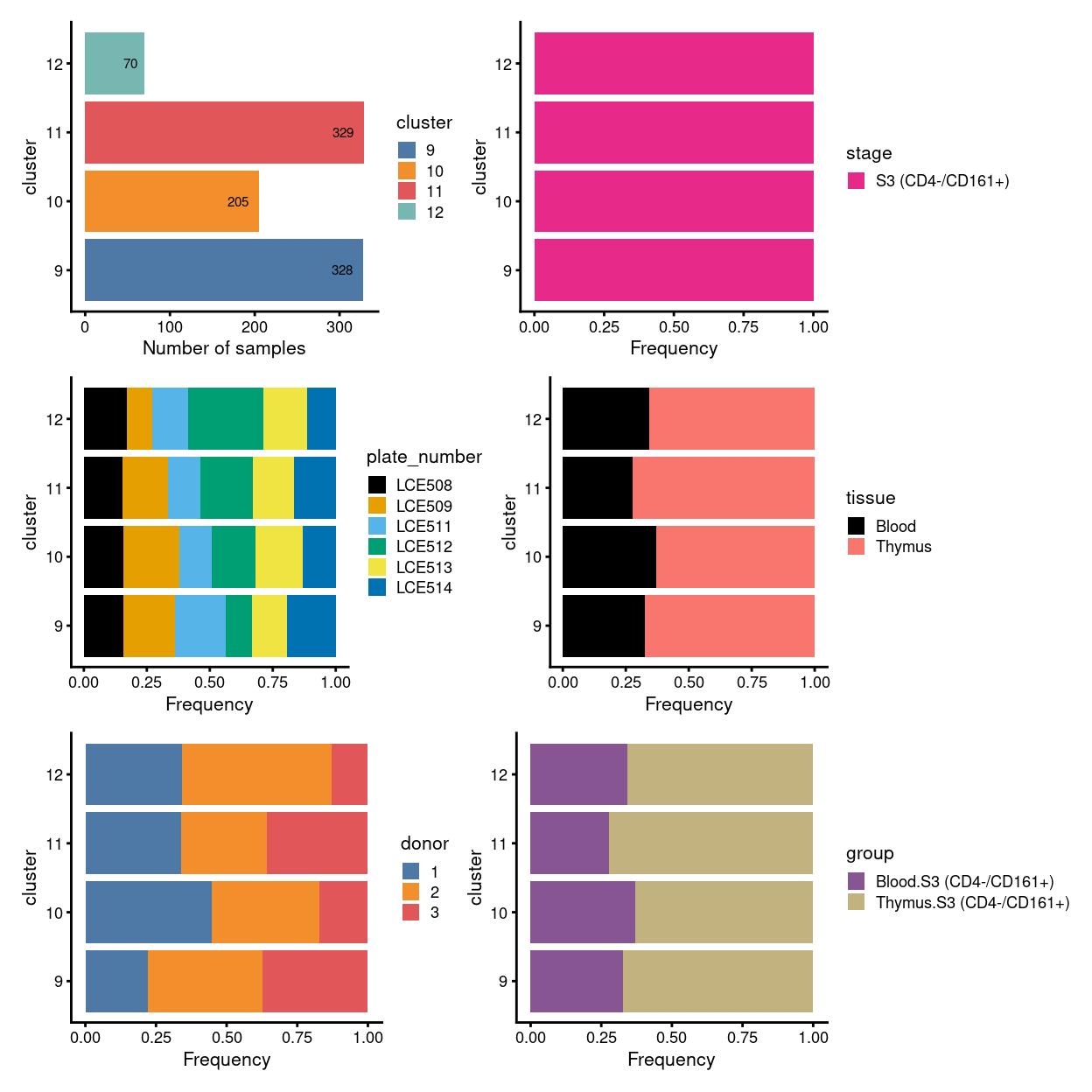
Figure 2: Breakdown of clusters by experimental factors.

PDF version of this figure is available in output/figures/cluster-barplot.single-cell.annotate.S3_only.pdf.

Show code

# NOTE: A potential figure for supplementary material.
pdf(
  here("output/figures/cluster-barplot.single-cell.annotate.S3_only.pdf"),
  height = 6, 
  width = 6)
(p1 | p2) / (p3 | p4) / (p5 | p6)
dev.off()

png 
  2 

Show code

dev.off()

null device 
          1 

NOTE: Considering the fact that SingleR with use of the annotation reference (Monaco Immune Cell Data) most relevant to the gamma-delta T cells (even annotated at cell level) could not further sub-classify the developmental stage/subtype of them (either annotating cluster as Th1 cell-/Naive CD8/CD4 T cell or Vd2gd T cells-alike) [ref: EDA_annotation_SingleR_MI_fine_cell_level.R], we decide to characterize the clusters by manual detection and curation of specific marker genes directly.

Marker gene detection

To interpret our clustering results, we identify the genes that drive separation between clusters. These marker genes allow us to assign biological meaning to each cluster based on their functional annotation. In the most obvious case, the marker genes for each cluster are a priori associated with particular cell types, allowing us to treat the clustering as a proxy for cell type identity. The same principle can be applied to more subtle differences in activation status or differentiation state.

Identification of marker genes is usually based around the retrospective detection of differential expression between clusters¹. Genes that are more strongly DE are more likely to have driven cluster separation in the first place. The top DE genes are likely to be good candidate markers as they can effectively distinguish between cells in different clusters.

The Welch t-test is an obvious choice of statistical method to test for differences in expression between clusters. It is quickly computed and has good statistical properties for large numbers of cells (Soneson and Robinson 2018).

Show code

# block on plate
sce$block <- paste0(sce$plate_number)

Cluster 9 vs. 10 vs. 11 vs. 12

Here we look for the unique up-regulated markers of each cluster when compared to the all remaining ones. For instance, unique markers of cluster 9 refer to the genes significantly up-regulated in all of these comparisons: cluster 10 vs. 9 and cluster 11 vs. 9 and cluster 12 vs. 9.

Show code

###################################
# (M1) raw unique
#
# cluster 9 (i.e. S3.mix.more.thymus.1) 
# cluster 10 (i.e. S3.mix.more.thymus.2) 
# cluster 11 (i.e. S3.mix.more.thymus.3)
# cluster 12 (i.e. S3.mix.more.thymus.4.center)

# find unique DE ./. clusters
uniquely_up <- findMarkers(
  sce,
  groups = sce$cluster,
  block = sce$block,
  pval.type = "all",
  direction = "up")

A PDF showing the top-20 markers in each cluster is shown in output/figures/heat-uniquely-up-logExp.annotate.S3_only.pdf.

Show code

# NOTE: A potential figure for supplementary material.
features <- lapply(uniquely_up, function(x) head(rownames(x), 20))
plotHeatmap(
  sce,
  features = unlist(features),
  columns = order(
    sce$cluster,
    sce$stage,
    sce$tissue,
    sce$donor,
    sce$group,
    sce$plate_number,
    sce$CD4,
    sce$CD161),
  colour_columns_by = c(
    "cluster",
    "stage",
    "tissue",
    "donor",
    "group",
    "plate_number",
    "CD4",
    "CD161"),
  cluster_cols = FALSE,
  center = TRUE,
  zlim = c(-3, 3),
  cluster_rows = FALSE,
  show_colnames = FALSE,
    annotation_row = data.frame(
    cluster = rep(names(features), lengths(features)),
    row.names = unlist(features)),
  column_annotation_colors = list(
    cluster = cluster_colours,
    stage = stage_colours,
    tissue = tissue_colours,
    donor = donor_colours,
    group = group_colours,
    plate_number = plate_number_colours),
  color = hcl.colors(101, "Blue-Red 3"),
  fontsize = 7,
  filename = here("output/figures/heat-uniquely-up-logExp.annotate.S3_only.pdf"),
  height = 12, 
  width = 10)

Show code

# export DGE lists
saveRDS(
  uniquely_up,
  here("data", "marker_genes", "S3_only", "C094_Pellicci.uniquely_up.cluster_9_vs_10_vs_11_vs_12.rds"),
  compress = "xz")

dir.create(here("output", "marker_genes", "S3_only", "uniquely_up", "cluster_9_vs_10_vs_11_vs_12"), recursive = TRUE)

vs_pair <- c("9", "10", "11", "12")

message("Writing 'uniquely_up (cluster_9_vs_10_vs_11_vs_12)' marker genes to file.")
for (n in names(uniquely_up)) {
  message(n)
  gzout <- gzfile(
    description = here(
      "output",
      "marker_genes",
      "S3_only",
      "uniquely_up",
      "cluster_9_vs_10_vs_11_vs_12",
      paste0("cluster_",
             vs_pair[which(names(uniquely_up) %in% n)],
             "_vs_",
             vs_pair[-which(names(uniquely_up) %in% n)][1],
             "_vs_",
             vs_pair[-which(names(uniquely_up) %in% n)][2],
             ".uniquely_up.csv.gz")),
    open = "wb")
  write.table(
    x = uniquely_up[[n]] %>%
      as.data.frame() %>%
      tibble::rownames_to_column("gene_ID"),
    file = gzout,
    sep = ",",
    quote = FALSE,
    row.names = FALSE,
    col.names = TRUE)
  close(gzout)
}

Show code

# NOTE: The following is a workaround to the lack of support for tabsets in 
#       distill (see https://github.com/rstudio/distill/issues/11 and 
#       https://github.com/rstudio/distill/issues/11#issuecomment-692142414 in 
#       particular).
xaringanExtra::use_panelset()

Cluster 9

Show code

##########################################
# look at cluster 9 (i.e. S3.mix.more.thymus.1)
chosen <- "9"
cluster9_uniquely_up <- uniquely_up[[chosen]]

# add description for the chosen cluster-group
x <- "(S3.mix.more.thymus.1)"

# look only at protein coding gene (pcg)
# NOTE: not suggest to narrow down into pcg as it remove all significant candidates (FDR << 0.05) !
# cluster9_uniquely_up <- cluster9_uniquely_up[intersect(protein_coding_gene_set, rownames(cluster9_uniquely_up)), ]

# get rid of noise (i.e. pseudo, ribo, mito, sex) that collaborator not interested in
cluster9_uniquely_up_noiseR <- cluster9_uniquely_up[setdiff(rownames(cluster9_uniquely_up), c(pseudogene_set, mito_set, ribo_set, sex_set)), ]

# see if key marker, "CD4 and/or ""KLRB1/CD161"", contain in the DE list + if it is "significant (i.e FDR <0.05)
y <- c("CD4",
       which(rownames(cluster9_uniquely_up_noiseR) %in% "CD4"),
       cluster9_uniquely_up_noiseR[which(rownames(cluster9_uniquely_up_noiseR) %in% "CD4"), ]$FDR < 0.05)
z <- c("KLRB1/CD161",
       which(rownames(cluster9_uniquely_up_noiseR) %in% "KLRB1"),
       cluster9_uniquely_up_noiseR[which(rownames(cluster9_uniquely_up_noiseR) %in% "KLRB1"), ]$FDR < 0.05)

# top25 only
best_set <- cluster9_uniquely_up_noiseR[1:25, ]

Show code

# heatmap
plotHeatmap(
  sce,
  features = rownames(best_set),
  columns = order(
    sce$cluster,
    sce$stage,
    sce$tissue,
    sce$donor,
    sce$group,
    sce$plate_number,
    sce$CD4,
    sce$CD161),
  colour_columns_by = c(
    "cluster",
    "stage",
    "tissue",
    "donor",
    "group",
    "plate_number",
    "CD4",
    "CD161"),
  cluster_cols = FALSE,
  center = TRUE,
  symmetric = TRUE,
  zlim = c(-3, 3),
  show_colnames = FALSE,
  annotation_row = data.frame(
    Sig = factor(
      ifelse(best_set[, "FDR"] < 0.05, "Yes", "No"),
      # TODO: temp trick to deal with the row-colouring problem
      # levels = c("Yes", "No")),
      levels = c("Yes")),
    row.names = rownames(best_set)),
  main = paste0("Cluster ", chosen, " ", x, " - \n",
                y[1], "_top ", y[2], "_significance: ", y[3], " ; \n",
                z[1], "_top ", z[2], "_significance: ", z[3]),
  column_annotation_colors = list(
    # Sig = c("Yes" = "red", "No" = "lightgrey"),
    cluster = cluster_colours,
    stage = stage_colours,
    tissue = tissue_colours,
    donor = donor_colours,
    group = group_colours,
    plate_number = plate_number_colours),
  color = hcl.colors(101, "Blue-Red 3"),
  fontsize = 7)

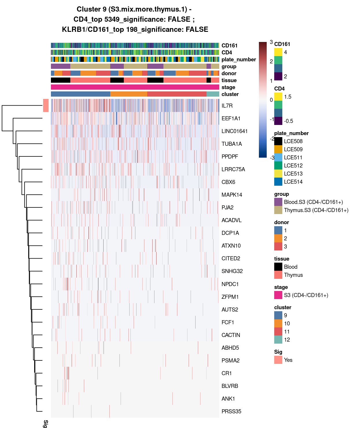
Figure 3: Heatmap of log-expression values in each sample for the top uniquely upregulated marker genes. Each column is a sample, each row a gene. Colours are capped at -3 and 3 to preserve dynamic range. Ranking of CD4 and CD161/KLRB1 from top of the DGE list sorted in ascending order of FDR and their statistical significance (TRUE = FDR < 0.05) are provided in the title

Cluster 10

Show code

##########################################
# look at cluster 7 (i.e. S3.mix.with.blood.1)
chosen <- "10"
cluster10_uniquely_up <- uniquely_up[[chosen]]

# add description for the chosen cluster-group
x <- "(S3.mix.more.thymus.2)"

# look only at protein coding gene (pcg)
# NOTE: not suggest to narrow down into pcg as it remove all significant candidates (FDR << 0.05) !
# cluster10_uniquely_up <- cluster10_uniquely_up[intersect(protein_coding_gene_set, rownames(cluster10_uniquely_up)), ]

# get rid of noise (i.e. pseudo, ribo, mito, sex) that collaborator not interested in
cluster10_uniquely_up_noiseR <- cluster10_uniquely_up[setdiff(rownames(cluster10_uniquely_up), c(pseudogene_set, mito_set, ribo_set, sex_set)), ]

# see if key marker, "CD4 and/or ""KLRB1/CD161"", contain in the DE list + if it is "significant (i.e FDR <0.05)
y <- c("CD4",
       which(rownames(cluster10_uniquely_up_noiseR) %in% "CD4"),
       cluster10_uniquely_up_noiseR[which(rownames(cluster10_uniquely_up_noiseR) %in% "CD4"), ]$FDR < 0.05)
z <- c("KLRB1/CD161",
       which(rownames(cluster10_uniquely_up_noiseR) %in% "KLRB1"),
       cluster10_uniquely_up_noiseR[which(rownames(cluster10_uniquely_up_noiseR) %in% "KLRB1"), ]$FDR < 0.05)

# top25 only
best_set <- cluster10_uniquely_up_noiseR[1:25, ]

Show code

# heatmap
plotHeatmap(
  sce,
  features = rownames(best_set),
  columns = order(
    sce$cluster,
    sce$stage,
    sce$tissue,
    sce$donor,
    sce$group,
    sce$plate_number,
    sce$CD4,
    sce$CD161),
  colour_columns_by = c(
    "cluster",
    "stage",
    "tissue",
    "donor",
    "group",
    "plate_number",
    "CD4",
    "CD161"),
  cluster_cols = FALSE,
  center = TRUE,
  symmetric = TRUE,
  zlim = c(-3, 3),
  show_colnames = FALSE,
  annotation_row = data.frame(
    Sig = factor(
      ifelse(best_set[, "FDR"] < 0.05, "Yes", "No"),
      # TODO: temp trick to deal with the row-colouring problem
      # levels = c("Yes", "No")),
      levels = c("Yes")),
    row.names = rownames(best_set)),
  main = paste0("Cluster ", chosen, " ", x, " - \n",
                y[1], "_top ", y[2], "_significance: ", y[3], " ; \n",
                z[1], "_top ", z[2], "_significance: ", z[3]),
  column_annotation_colors = list(
    # Sig = c("Yes" = "red", "No" = "lightgrey"),
    cluster = cluster_colours,
    stage = stage_colours,
    tissue = tissue_colours,
    donor = donor_colours,
    group = group_colours,
    plate_number = plate_number_colours),
  color = hcl.colors(101, "Blue-Red 3"),
  fontsize = 7)

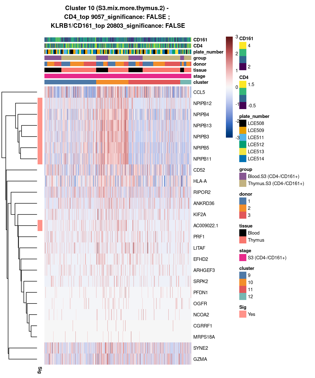
Figure 4: Heatmap of log-expression values in each sample for the top uniquely upregulated marker genes. Each column is a sample, each row a gene. Colours are capped at -3 and 3 to preserve dynamic range. Ranking of CD4 and CD161/KLRB1 from top of the DGE list sorted in ascending order of FDR and their statistical significance (TRUE = FDR < 0.05) are provided in the title

Cluster 11

Show code

##########################################
# look at cluster 11 (i.e. S3.mix.more.thymus.3)
chosen <- "11"
cluster11_uniquely_up <- uniquely_up[[chosen]]

# add description for the chosen cluster-group
x <- "(S3.mix.more.thymus.3)"

# look only at protein coding gene (pcg)
# NOTE: not suggest to narrow down into pcg as it remove all significant candidates (FDR << 0.05) !
# cluster11_uniquely_up <- cluster11_uniquely_up[intersect(protein_coding_gene_set, rownames(cluster11_uniquely_up)), ]

# get rid of noise (i.e. pseudo, ribo, mito, sex) that collaborator not interested in
cluster11_uniquely_up_noiseR <- cluster11_uniquely_up[setdiff(rownames(cluster11_uniquely_up), c(pseudogene_set, mito_set, ribo_set, sex_set)), ]

# see if key marker, "CD4 and/or ""KLRB1/CD161"", contain in the DE list + if it is "significant (i.e FDR <0.05)
y <- c("CD4",
       which(rownames(cluster11_uniquely_up_noiseR) %in% "CD4"),
       cluster11_uniquely_up_noiseR[which(rownames(cluster11_uniquely_up_noiseR) %in% "CD4"), ]$FDR < 0.05)
z <- c("KLRB1/CD161",
       which(rownames(cluster11_uniquely_up_noiseR) %in% "KLRB1"),
       cluster11_uniquely_up_noiseR[which(rownames(cluster11_uniquely_up_noiseR) %in% "KLRB1"), ]$FDR < 0.05)

# top25 only
best_set <- cluster11_uniquely_up_noiseR[1:25, ]

Show code

# heatmap
plotHeatmap(
  sce,
  features = rownames(best_set),
  columns = order(
    sce$cluster,
    sce$stage,
    sce$tissue,
    sce$donor,
    sce$group,
    sce$plate_number,
    sce$CD4,
    sce$CD161),
  colour_columns_by = c(
    "cluster",
    "stage",
    "tissue",
    "donor",
    "group",
    "plate_number",
    "CD4",
    "CD161"),
  cluster_cols = FALSE,
  center = TRUE,
  symmetric = TRUE,
  zlim = c(-3, 3),
  show_colnames = FALSE,
  # annotation_row = data.frame(
  #   Sig = factor(
  #     ifelse(best_set[, "FDR"] < 0.05, "Yes", "No"),
  #     # TODO: temp trick to deal with the row-colouring problem
  #     # levels = c("Yes", "No")),
  #     levels = c("Yes")),
  #   row.names = rownames(best_set)),
  main = paste0("Cluster ", chosen, " ", x, " - \n",
                y[1], "_top ", y[2], "_significance: ", y[3], " ; \n",
                z[1], "_top ", z[2], "_significance: ", z[3]),
  column_annotation_colors = list(
    # Sig = c("Yes" = "red", "No" = "lightgrey"),
    cluster = cluster_colours,
    stage = stage_colours,
    tissue = tissue_colours,
    donor = donor_colours,
    group = group_colours,
    plate_number = plate_number_colours),
  color = hcl.colors(101, "Blue-Red 3"),
  fontsize = 7)

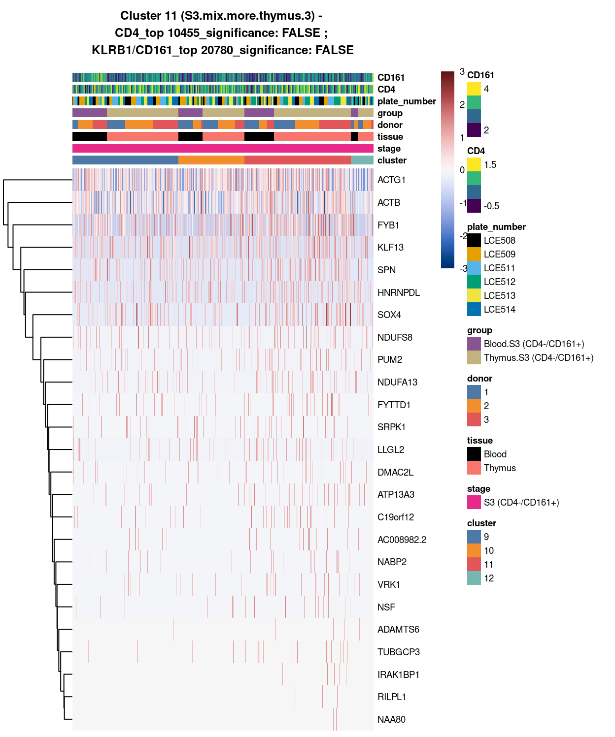
Figure 5: Heatmap of log-expression values in each sample for the top uniquely upregulated marker genes. Each column is a sample, each row a gene. Colours are capped at -3 and 3 to preserve dynamic range. Ranking of CD4 and CD161/KLRB1 from top of the DGE list sorted in ascending order of FDR and their statistical significance (TRUE = FDR < 0.05) are provided in the title

Cluster 12

Show code

##########################################
# look at cluster 12 (i.e. S3.mix.more.thymus.4.center)
chosen <- "12"
cluster12_uniquely_up <- uniquely_up[[chosen]]

# add description for the chosen cluster-group
x <- "(S3.mix.more.thymus.4.center)"

# look only at protein coding gene (pcg)
# NOTE: not suggest to narrow down into pcg as it remove all significant candidates (FDR << 0.05) !
# cluster12_uniquely_up <- cluster12_uniquely_up[intersect(protein_coding_gene_set, rownames(cluster12_uniquely_up)), ]

# get rid of noise (i.e. pseudo, ribo, mito, sex) that collaborator not interested in
cluster12_uniquely_up_noiseR <- cluster12_uniquely_up[setdiff(rownames(cluster12_uniquely_up), c(pseudogene_set, mito_set, ribo_set, sex_set)), ]

# see if key marker, "CD4 and/or ""KLRB1/CD161"", contain in the DE list + if it is "significant (i.e FDR <0.05)
y <- c("CD4",
       which(rownames(cluster12_uniquely_up_noiseR) %in% "CD4"),
       cluster12_uniquely_up_noiseR[which(rownames(cluster12_uniquely_up_noiseR) %in% "CD4"), ]$FDR < 0.05)
z <- c("KLRB1/CD161",
       which(rownames(cluster12_uniquely_up_noiseR) %in% "KLRB1"),
       cluster12_uniquely_up_noiseR[which(rownames(cluster12_uniquely_up_noiseR) %in% "KLRB1"), ]$FDR < 0.05)

# top25 only
best_set <- cluster12_uniquely_up_noiseR[1:25, ]

Show code

# heatmap
plotHeatmap(
  sce,
  features = rownames(best_set),
  columns = order(
    sce$cluster,
    sce$stage,
    sce$tissue,
    sce$donor,
    sce$group,
    sce$plate_number,
    sce$CD4,
    sce$CD161),
  colour_columns_by = c(
    "cluster",
    "stage",
    "tissue",
    "donor",
    "group",
    "plate_number",
    "CD4",
    "CD161"),
  cluster_cols = FALSE,
  center = TRUE,
  symmetric = TRUE,
  zlim = c(-3, 3),
  show_colnames = FALSE,
  # annotation_row = data.frame(
  #   Sig = factor(
  #     ifelse(best_set[, "FDR"] < 0.05, "Yes", "No"),
  #     # TODO: temp trick to deal with the row-colouring problem
  #     # levels = c("Yes", "No")),
  #     levels = c("Yes")),
  #   row.names = rownames(best_set)),
  main = paste0("Cluster ", chosen, " ", x, " - \n",
                y[1], "_top ", y[2], "_significance: ", y[3], " ; \n",
                z[1], "_top ", z[2], "_significance: ", z[3]),
  column_annotation_colors = list(
    # Sig = c("Yes" = "red", "No" = "lightgrey"),
    cluster = cluster_colours,
    stage = stage_colours,
    tissue = tissue_colours,
    donor = donor_colours,
    group = group_colours,
    plate_number = plate_number_colours),
  color = hcl.colors(101, "Blue-Red 3"),
  fontsize = 7)

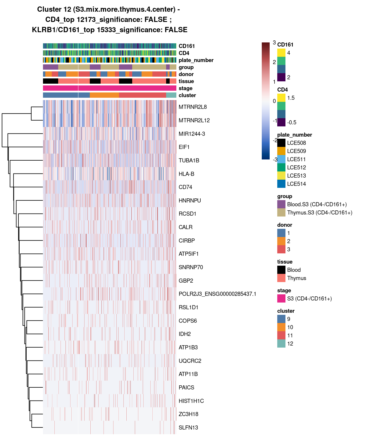
Figure 6: Heatmap of log-expression values in each sample for the top uniquely upregulated marker genes. Each column is a sample, each row a gene. Colours are capped at -3 and 3 to preserve dynamic range. Ranking of CD4 and CD161/KLRB1 from top of the DGE list sorted in ascending order of FDR and their statistical significance (TRUE = FDR < 0.05) are provided in the title

DGE lists of these comparisons are available in output/marker_genes/S3_only/uniquely_up/cluster_9_vs_10_vs_11_vs_12/.

Summary:

IL7R is the clear and only unique marker of cluster 9. Cluster 10 also got number of NPBIB family members as marker, but if exclude them, AC009022.1 is the only global unique marker of this clusters. For cluster 11, no statistically significant marker can be spotted, but visually, genes like SOX4 seems to be a potential candidate if pairwise compare. Cluster 12 is the cluster located at the center and be surrounded by the other three clusters in the UMAP plot, as expected, we cannot find any globally unique markers for it.

With this regard, apart from making “all pairwise comparisons” between “all clusters” to pinpoint DE unique to each cluster as above, we took an alternative path and determined the DE unique to only the “selected pairwise comparisons” between “clusters” below. Say, for cluster 12, we determine markers that is significantly up-regulated in at least one of these comparisons: cluster 9 vs. 12 or cluster 10 vs. 12 or cluster 11 vs. 12.

Besides, we also look into the the pairwise comparisons between the interesting “cluster-groups”. For instance, as all cluster has a similar composition of S3-mix with higher proportion of thymus cells, it would be interesting to know how cluster 9, 10, 11 are different from each other, or if we could trace for the feature or role of the centered cluster 12 if we pairwise compare it with the rest.

Here are the list of pairwise comparisons and what they are anticipated to achieve when compared:

fx: are these four clusters really differernt from each other individually

• 9 vs 10 (A vs B)
• 9 vs 11 (C vs D)
• 9 vs 12 (E vs F)
• 10 vs 11 (G vs H)
• 10 vs 12 (I vs J)
• 11 vs 12 (K vs L)

fx: how different between clusters at the peripheral

• 9_10 vs 11 (M vs N)
• 10_11 vs 9 (O vs P)
• 9_11 vs 10 (Q vs R)

fx: combined peripheral clusters compare with the central cluster

• 9_10 vs 12 (S vs T)
• 10_11 vs 12 (U vs V)
• 9_11 vs 12 (W vs X)
• 9_10_11 vs 12 (Y vs Z)

Selected pairwise comparisons

Show code

# NOTE: The following is a workaround to the lack of support for tabsets in 
#       distill (see https://github.com/rstudio/distill/issues/11 and 
#       https://github.com/rstudio/distill/issues/11#issuecomment-692142414 in 
#       particular).
xaringanExtra::use_panelset()

cluster_9_vs_cluster_10

Show code

#########
# A vs B
#########

##########################################################################################
# cluster 9 (i.e. S3.mix.more.thymus.1) vs cluster 10 (i.e. S3.mix.more.thymus.2)

# checkpoint
cp <- sce
# exclude cells of uninterested cluster from cp
cp <- cp[, cp$cluster == "9" | cp$cluster == "10"]
colData(cp) <- droplevels(colData(cp))

# classify cluster-group for comparison
cp$vs1 <- factor(ifelse(cp$cluster == 9, "A", "B"))

# set vs colours
vs1_colours <- setNames(
  palette.colors(nlevels(cp$vs1), "Set1"),
  levels(cp$vs1))
cp$colours$vs1_colours <- vs1_colours[cp$vs1]

# find unique DE ./. cluster-groups
vs1_uniquely_up <- findMarkers(
  cp,
  groups = cp$vs1,
  block = cp$block,
  pval.type = "all",
  direction = "up")

# export DGE lists
saveRDS(
  vs1_uniquely_up,
  here("data", "marker_genes", "S3_only", "C094_Pellicci.uniquely_up.cluster_9_vs_10.rds"),
  compress = "xz")

dir.create(here("output", "marker_genes", "S3_only", "uniquely_up", "cluster_9_vs_10"), recursive = TRUE)

vs_pair <- c("9", "10")

message("Writing 'uniquely_up (cluster_9_vs_10)' marker genes to file.")
for (n in names(vs1_uniquely_up)) {
  message(n)
  gzout <- gzfile(
    description = here(
      "output",
      "marker_genes",
      "S3_only",
      "uniquely_up",
      "cluster_9_vs_10",
      paste0("cluster_",
             vs_pair[which(names(vs1_uniquely_up) %in% n)],
             "_vs_",
             vs_pair[-which(names(vs1_uniquely_up) %in% n)][1],
             ".uniquely_up.csv.gz")),
    open = "wb")
  write.table(
    x = vs1_uniquely_up[[n]] %>%
      as.data.frame() %>%
      tibble::rownames_to_column("gene_ID"),
    file = gzout,
    sep = ",",
    quote = FALSE,
    row.names = FALSE,
    col.names = TRUE)
  close(gzout)
}

Show code

###############################################################
# look at cluster-group A / cluster 9 (i.e. S3.mix.more.thymus.1)
chosen <- "A"
A_uniquely_up <- vs1_uniquely_up[[chosen]]

# add description for the chosen cluster-group
x <- "(cluster 9; S3.mix.more.thymus.1)"

# look only at protein coding gene (pcg)
# NOTE: not suggest to narrow down into pcg as it remove all significant candidates (FDR << 0.05) !
# A_uniquely_up_pcg <- A_uniquely_up[intersect(protein_coding_gene_set, rownames(A_uniquely_up)), ]

# get rid of noise (i.e. pseudo, ribo, mito, sex) that collaborator not interested in
A_uniquely_up_noiseR <- A_uniquely_up[setdiff(rownames(A_uniquely_up), c(pseudogene_set, mito_set, ribo_set, sex_set)), ]

# see if key marker, "CD4 and/or ""KLRB1/CD161"", contain in the DE list + if it is "significant (i.e FDR <0.05)
y <- c("CD4",
       which(rownames(A_uniquely_up_noiseR) %in% "CD4"),
       A_uniquely_up_noiseR[which(rownames(A_uniquely_up_noiseR) %in% "CD4"), ]$FDR < 0.05)
z <- c("KLRB1/CD161",
       which(rownames(A_uniquely_up_noiseR) %in% "KLRB1"),
       A_uniquely_up_noiseR[which(rownames(A_uniquely_up_noiseR) %in% "KLRB1"), ]$FDR < 0.05)

# top25 only + gene-of-interest
best_set <- A_uniquely_up_noiseR[1:25, ]

Show code

# heatmap
plotHeatmap(
  cp,
  features = rownames(best_set),
  columns = order(
    cp$vs1,
    cp$cluster,
    cp$stage,
    cp$tissue,
    cp$donor,
    cp$group,
    cp$plate_number,
    cp$CD4,
    cp$CD161),
  colour_columns_by = c(
    "vs1",
    "cluster",
    "stage",
    "tissue",
    "donor",
    "group",
    "plate_number",
    "CD4",
    "CD161"),
  cluster_cols = FALSE,
  center = TRUE,
  symmetric = TRUE,
  zlim = c(-3, 3),
  show_colnames = FALSE,
  annotation_row = data.frame(
    Sig = factor(
      ifelse(best_set[, "FDR"] < 0.05, "Yes", "No"),
      # TODO: temp trick to deal with the row-colouring problem
      # levels = c("Yes", "No")),
      levels = c("Yes")),
    row.names = rownames(best_set)),
  main = paste0("Cluster-group: ", chosen, " ", x, " - \n",
                y[1], "_top ", y[2], "_significance: ", y[3], " ; \n",
                z[1], "_top ", z[2], "_significance: ", z[3]),
  column_annotation_colors = list(
    # Sig = c("Yes" = "red", "No" = "lightgrey"),
    vs1 = vs1_colours,
    cluster = cluster_colours,
    stage = stage_colours,
    tissue = tissue_colours,
    donor = donor_colours,
    group = group_colours,
    plate_number = plate_number_colours),
  color = hcl.colors(101, "Blue-Red 3"),
  fontsize = 7)

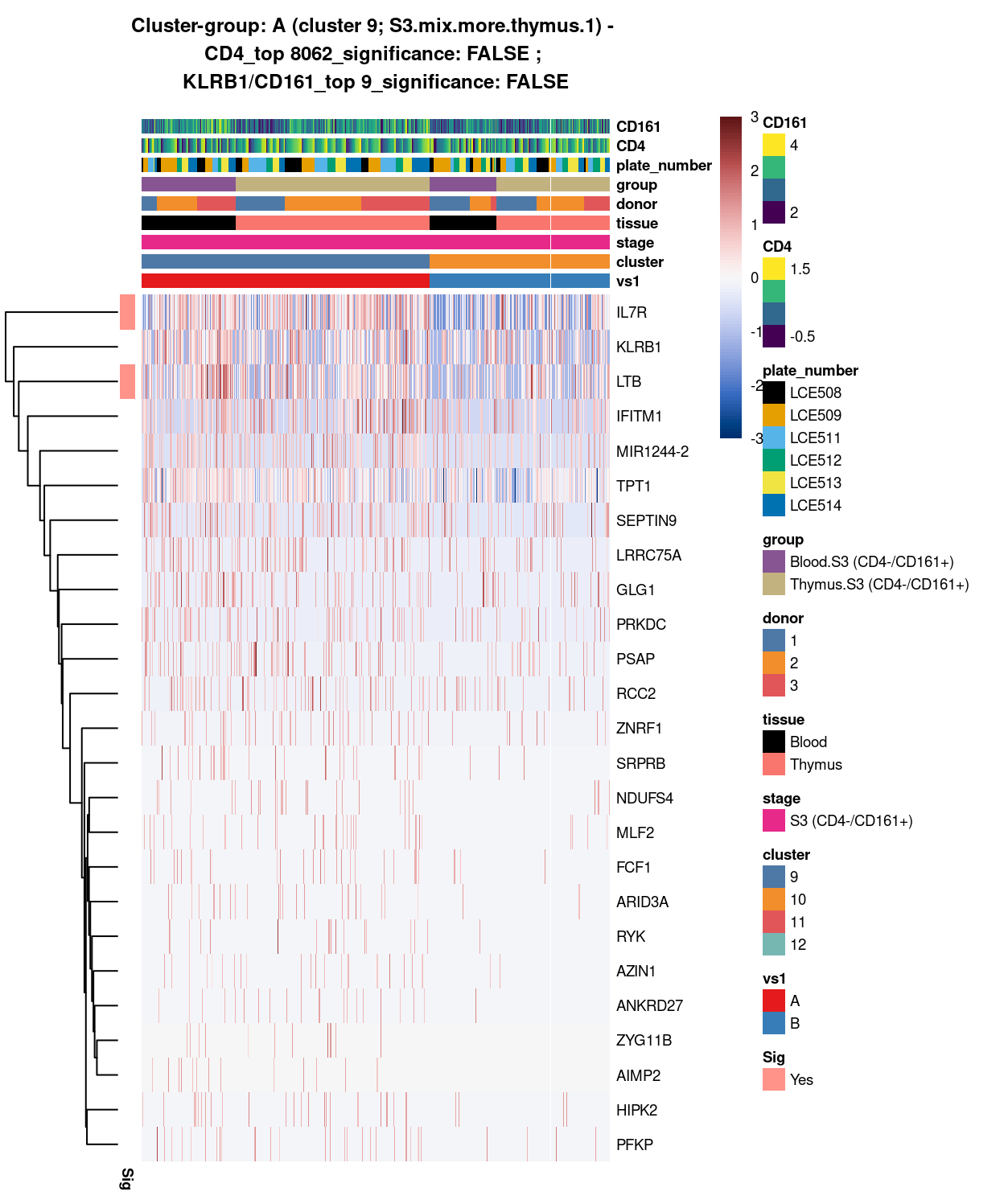
Figure 7: Heatmap of log-expression values in each sample for the top uniquely upregulated marker genes. Each column is a sample, each row a gene. Colours are capped at -3 and 3 to preserve dynamic range. Ranking of CD4 and CD161/KLRB1 from top of the DGE list sorted in ascending order of FDR and their statistical significance (TRUE = FDR < 0.05) are provided in the title.

Show code

##########################################################
# look at cluster-group B / cluster 10 (i.e. S3.mix.more.thymus.2)
chosen <- "B"
B_uniquely_up <- vs1_uniquely_up[[chosen]]

# add description for the chosen cluster-group
x <- "(cluster 10; S3.mix.more.thymus.2)"

# look only at protein coding gene (pcg)
# NOTE: not suggest to narrow down into pcg as it remove all significant candidates (FDR << 0.05) !
# B_uniquely_up_pcg <- B_uniquely_up[intersect(protein_coding_gene_set, rownames(B_uniquely_up)), ]

# get rid of noise (i.e. pseudo, ribo, mito, sex) that collaborator not interested in
B_uniquely_up_noiseR <- B_uniquely_up[setdiff(rownames(B_uniquely_up), c(pseudogene_set, mito_set, ribo_set, sex_set)), ]

# see if key marker, "CD4 and/or ""KLRB1/CD161"", contain in the DE list + if it is "significant (i.e FDR <0.05)
y <- c("CD4",
       which(rownames(B_uniquely_up_noiseR) %in% "CD4"),
       B_uniquely_up_noiseR[which(rownames(B_uniquely_up_noiseR) %in% "CD4"), ]$FDR < 0.05)
z <- c("KLRB1/CD161",
       which(rownames(B_uniquely_up_noiseR) %in% "KLRB1"),
       B_uniquely_up_noiseR[which(rownames(B_uniquely_up_noiseR) %in% "KLRB1"), ]$FDR < 0.05)

# top25 only + gene-of-interest
best_set <- B_uniquely_up_noiseR[1:25, ]

Show code

# heatmap
plotHeatmap(
  cp,
  features = rownames(best_set),
  columns = order(
    cp$vs1,
    cp$cluster,
    cp$stage,
    cp$tissue,
    cp$donor,
    cp$group,
    cp$plate_number,
    cp$CD4,
    cp$CD161),
  colour_columns_by = c(
    "vs1",
    "cluster",
    "stage",
    "tissue",
    "donor",
    "group",
    "plate_number",
    "CD4",
    "CD161"),
  cluster_cols = FALSE,
  center = TRUE,
  symmetric = TRUE,
  zlim = c(-3, 3),
  show_colnames = FALSE,
  annotation_row = data.frame(
    Sig = factor(
      ifelse(best_set[, "FDR"] < 0.05, "Yes", "No"),
      # TODO: temp trick to deal with the row-colouring problem
      # levels = c("Yes", "No")),
      levels = c("Yes")),
    row.names = rownames(best_set)),
  main = paste0("Cluster-group: ", chosen, " ", x, " - \n",
                y[1], "_top ", y[2], "_significance: ", y[3], " ; \n",
                z[1], "_top ", z[2], "_significance: ", z[3]),
  column_annotation_colors = list(
    # Sig = c("Yes" = "red", "No" = "lightgrey"),
    vs1 = vs1_colours,
    cluster = cluster_colours,
    stage = stage_colours,
    tissue = tissue_colours,
    donor = donor_colours,
    group = group_colours,
    plate_number = plate_number_colours),
  color = hcl.colors(101, "Blue-Red 3"),
  fontsize = 7)

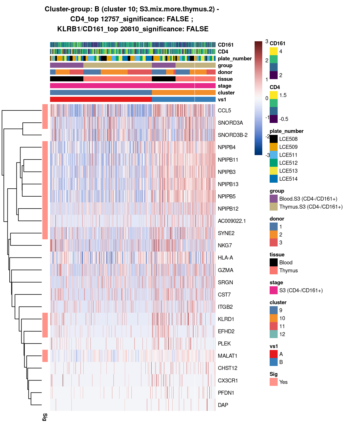
Figure 8: Heatmap of log-expression values in each sample for the top uniquely upregulated marker genes. Each column is a sample, each row a gene. Colours are capped at -3 and 3 to preserve dynamic range. Ranking of CD4 and CD161/KLRB1 from top of the DGE list sorted in ascending order of FDR and their statistical significance (TRUE = FDR < 0.05) are provided in the title.

DGE lists of these comparisons are available in output/marker_genes/S3_only/uniquely_up/cluster_9_vs_10/.

SUMMARY: 9 vs 10 (A vs B)

• cluster 9 (S3.mix.more.thymus.1 >>> IL7R and LTB as the only markers; DE not associated with tissue
• cluster 10 (S3.mix.more.thymus.2 >>> besides NPIPB family, number of markers found (e.g. CCL5 and SYNE2 for both tissues; KLRD1 and EFHD2 mostly for blood)
• COMMENT: they are two separated subtype S3 cells found in both thymus and blood (where cluster 9 si characterized by higher IL7R and LTB expression)

cluster_9_vs_cluster_11

Show code

#########
# C vs D
#########

##########################################################################################
# cluster 9 (i.e. S3.mix.more.thymus.1) vs cluster 11 (i.e. S3.mix.more.thymus.3)

# checkpoint
cp <- sce
# exclude cells of uninterested cluster from cp
cp <- cp[, cp$cluster == "9" | cp$cluster == "11"]
colData(cp) <- droplevels(colData(cp))

# classify cluster-group for comparison
cp$vs2 <- factor(ifelse(cp$cluster == 9, "C", "D"))

# set vs colours
vs2_colours <- setNames(
  palette.colors(nlevels(cp$vs2), "Set1"),
  levels(cp$vs2))
cp$colours$vs2_colours <- vs2_colours[cp$vs2]

# find unique DE ./. cluster-groups
vs2_uniquely_up <- findMarkers(
  cp,
  groups = cp$vs2,
  block = cp$block,
  pval.type = "all",
  direction = "up")

# export DGE lists
saveRDS(
  vs2_uniquely_up,
  here("data", "marker_genes", "S3_only", "C094_Pellicci.uniquely_up.cluster_9_vs_11.rds"),
  compress = "xz")

dir.create(here("output", "marker_genes", "S3_only", "uniquely_up", "cluster_9_vs_11"), recursive = TRUE)

vs_pair <- c("9", "11")

message("Writing 'uniquely_up (cluster_9_vs_11)' marker genes to file.")
for (n in names(vs2_uniquely_up)) {
  message(n)
  gzout <- gzfile(
    description = here(
      "output",
      "marker_genes",
      "S3_only",
      "uniquely_up",
      "cluster_9_vs_11",
      paste0("cluster_",
             vs_pair[which(names(vs2_uniquely_up) %in% n)],
             "_vs_",
             vs_pair[-which(names(vs2_uniquely_up) %in% n)][1],
             ".uniquely_up.csv.gz")),
    open = "wb")
  write.table(
    x = vs2_uniquely_up[[n]] %>%
      as.data.frame() %>%
      tibble::rownames_to_column("gene_ID"),
    file = gzout,
    sep = ",",
    quote = FALSE,
    row.names = FALSE,
    col.names = TRUE)
  close(gzout)
}

Show code

###############################################################
# look at cluster-group C / cluster 9 (i.e. S3.mix.more.thymus.1)
chosen <- "C"
C_uniquely_up <- vs2_uniquely_up[[chosen]]

# add description for the chosen cluster-group
x <- "(cluster 9; S3.mix.more.thymus.1)"

# look only at protein coding gene (pcg)
# NOTE: not suggest to narrow down into pcg as it remove all significant candidates (FDR << 0.05) !
# C_uniquely_up_pcg <- C_uniquely_up[intersect(protein_coding_gene_set, rownames(C_uniquely_up)), ]

# get rid of noise (i.e. pseudo, ribo, mito, sex) that collaborator not interested in
C_uniquely_up_noiseR <- C_uniquely_up[setdiff(rownames(C_uniquely_up), c(pseudogene_set, mito_set, ribo_set, sex_set)), ]

# see if key marker, "CD4 and/or ""KLRB1/CD161"", contain in the DE list + if it is "significant (i.e FDR <0.05)
y <- c("CD4",
       which(rownames(C_uniquely_up_noiseR) %in% "CD4"),
       C_uniquely_up_noiseR[which(rownames(C_uniquely_up_noiseR) %in% "CD4"), ]$FDR < 0.05)
z <- c("KLRB1/CD161",
       which(rownames(C_uniquely_up_noiseR) %in% "KLRB1"),
       C_uniquely_up_noiseR[which(rownames(C_uniquely_up_noiseR) %in% "KLRB1"), ]$FDR < 0.05)

# top25 only + gene-of-interest
best_set <- C_uniquely_up_noiseR[1:25, ]

Show code

# heatmap
plotHeatmap(
  cp,
  features = rownames(best_set),
  columns = order(
    cp$vs2,
    cp$cluster,
    cp$stage,
    cp$tissue,
    cp$donor,
    cp$group,
    cp$plate_number,
    cp$CD4,
    cp$CD161),
  colour_columns_by = c(
    "vs2",
    "cluster",
    "stage",
    "tissue",
    "donor",
    "group",
    "plate_number",
    "CD4",
    "CD161"),
  cluster_cols = FALSE,
  center = TRUE,
  symmetric = TRUE,
  zlim = c(-3, 3),
  show_colnames = FALSE,
  annotation_row = data.frame(
    Sig = factor(
      ifelse(best_set[, "FDR"] < 0.05, "Yes", "No"),
      # TODO: temp trick to deal with the row-colouring problem
      # levels = c("Yes", "No")),
      levels = c("Yes")),
    row.names = rownames(best_set)),
  main = paste0("Cluster-group: ", chosen, " ", x, " - \n",
                y[1], "_top ", y[2], "_significance: ", y[3], " ; \n",
                z[1], "_top ", z[2], "_significance: ", z[3]),
  column_annotation_colors = list(
    # Sig = c("Yes" = "red", "No" = "lightgrey"),
    vs2 = vs2_colours,
    cluster = cluster_colours,
    stage = stage_colours,
    tissue = tissue_colours,
    donor = donor_colours,
    group = group_colours,
    plate_number = plate_number_colours),
  color = hcl.colors(101, "Blue-Red 3"),
  fontsize = 7)

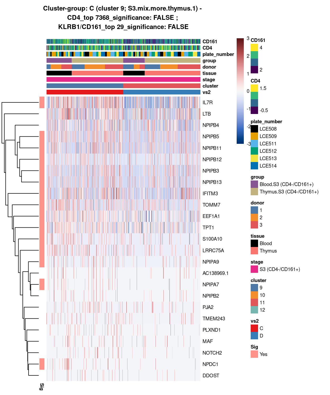
Figure 9: Heatmap of log-expression values in each sample for the top uniquely upregulated marker genes. Each column is a sample, each row a gene. Colours are capped at -3 and 3 to preserve dynamic range. Ranking of CD4 and CD161/KLRB1 from top of the DGE list sorted in ascending order of FDR and their statistical significance (TRUE = FDR < 0.05) are provided in the title.

Show code

##########################################################
# look at cluster-group D / cluster 11 (i.e. S3.mix.more.thymus.3)
chosen <- "D"
D_uniquely_up <- vs2_uniquely_up[[chosen]]

# add description for the chosen cluster-group
x <- "(cluster 11; S3.mix.more.thymus.3)"

# look only at protein coding gene (pcg)
# NOTE: not suggest to narrow down into pcg as it remove all significant candidates (FDR << 0.05) !
# D_uniquely_up_pcg <- D_uniquely_up[intersect(protein_coding_gene_set, rownames(D_uniquely_up)), ]

# get rid of noise (i.e. pseudo, ribo, mito, sex) that collaborator not interested in
D_uniquely_up_noiseR <- D_uniquely_up[setdiff(rownames(D_uniquely_up), c(pseudogene_set, mito_set, ribo_set, sex_set)), ]

# see if key marker, "CD4 and/or ""KLRB1/CD161"", contain in the DE list + if it is "significant (i.e FDR <0.05)
y <- c("CD4",
       which(rownames(D_uniquely_up_noiseR) %in% "CD4"),
       D_uniquely_up_noiseR[which(rownames(D_uniquely_up_noiseR) %in% "CD4"), ]$FDR < 0.05)
z <- c("KLRB1/CD161",
       which(rownames(D_uniquely_up_noiseR) %in% "KLRB1"),
       D_uniquely_up_noiseR[which(rownames(D_uniquely_up_noiseR) %in% "KLRB1"), ]$FDR < 0.05)

# top25 only + gene-of-interest
best_set <- D_uniquely_up_noiseR[1:25, ]

Show code

# heatmap
plotHeatmap(
  cp,
  features = rownames(best_set),
  columns = order(
    cp$vs2,
    cp$cluster,
    cp$stage,
    cp$tissue,
    cp$donor,
    cp$group,
    cp$plate_number,
    cp$CD4,
    cp$CD161),
  colour_columns_by = c(
    "vs2",
    "cluster",
    "stage",
    "tissue",
    "donor",
    "group",
    "plate_number",
    "CD4",
    "CD161"),
  cluster_cols = FALSE,
  center = TRUE,
  symmetric = TRUE,
  zlim = c(-3, 3),
  show_colnames = FALSE,
  annotation_row = data.frame(
    Sig = factor(
      ifelse(best_set[, "FDR"] < 0.05, "Yes", "No"),
      # TODO: temp trick to deal with the row-colouring problem
      # levels = c("Yes", "No")),
      levels = c("Yes")),
    row.names = rownames(best_set)),
  main = paste0("Cluster-group: ", chosen, " ", x, " - \n",
                y[1], "_top ", y[2], "_significance: ", y[3], " ; \n",
                z[1], "_top ", z[2], "_significance: ", z[3]),
  column_annotation_colors = list(
    # Sig = c("Yes" = "red", "No" = "lightgrey"),
    vs2 = vs2_colours,
    cluster = cluster_colours,
    stage = stage_colours,
    tissue = tissue_colours,
    donor = donor_colours,
    group = group_colours,
    plate_number = plate_number_colours),
  color = hcl.colors(101, "Blue-Red 3"),
  fontsize = 7)

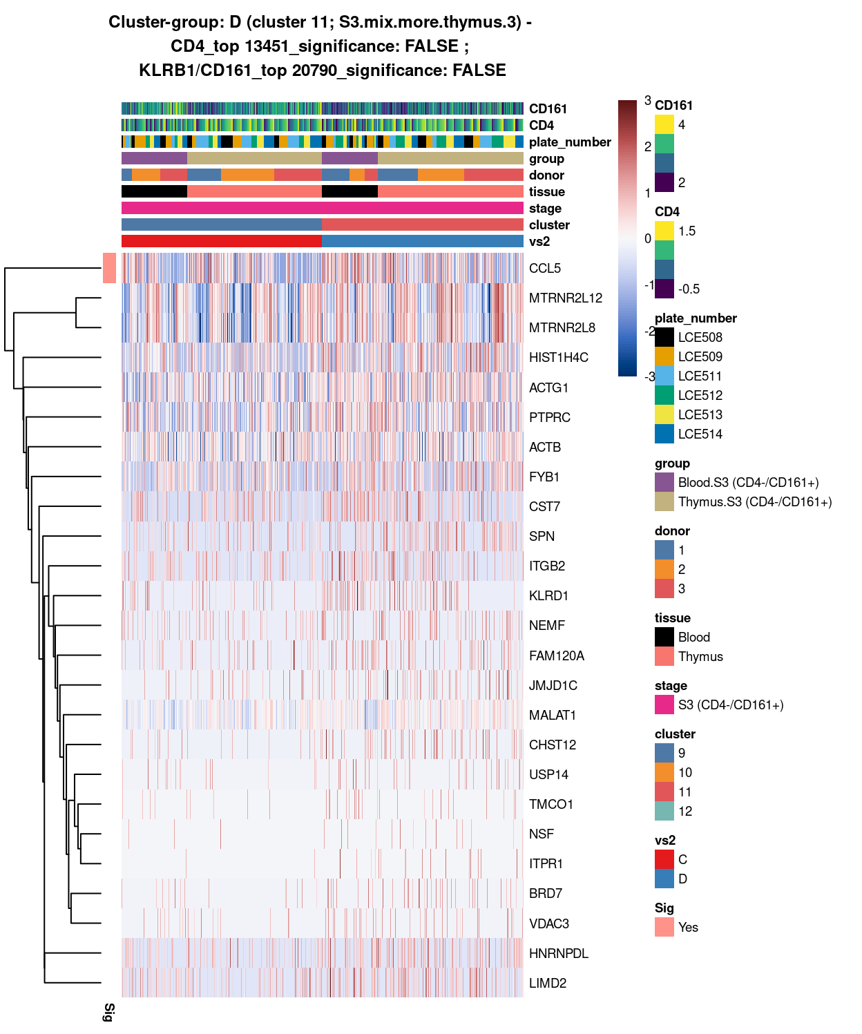
Figure 10: Heatmap of log-expression values in each sample for the top uniquely upregulated marker genes. Each column is a sample, each row a gene. Colours are capped at -3 and 3 to preserve dynamic range. Ranking of CD4 and CD161/KLRB1 from top of the DGE list sorted in ascending order of FDR and their statistical significance (TRUE = FDR < 0.05) are provided in the title.

DGE lists of these comparisons are available in output/marker_genes/S3_only/uniquely_up/cluster_9_vs_11/.

SUMMARY: 9 vs 11 (C vs D)

• cluster 9 (S3.mix.more.thymus.1 >>> besides NPIPB family, number of markers such as IL7R, IFITM3, TOMM7, etc shown as clear markers
• cluster 11 (S3.mix.more.thymus.3 >>> CCL5 as only unique makers (may look more highly expressed in “blood” cells)
• COMMENT: these are also 2 separated subtypes of S3 cells (esp cluster 9 is IL7R IFITM3 driven, cluster 11 is CCL5 driven

cluster_9_vs_cluster_12

Show code

#########
# E vs F
#########

##########################################################################################
# cluster 9 (i.e. S3.mix.more.thymus.1) vs cluster 12 (i.e. S3.mix.more.thymus.4.center)

# checkpoint
cp <- sce
# exclude cells of uninterested cluster from cp
cp <- cp[, cp$cluster == "9" | cp$cluster == "12"]
colData(cp) <- droplevels(colData(cp))

# classify cluster-group for comparison
cp$vs3 <- factor(ifelse(cp$cluster == 9, "E", "F"))

# set vs colours
vs3_colours <- setNames(
  palette.colors(nlevels(cp$vs3), "Set1"),
  levels(cp$vs3))
cp$colours$vs3_colours <- vs3_colours[cp$vs3]

# find unique DE ./. cluster-groups
vs3_uniquely_up <- findMarkers(
  cp,
  groups = cp$vs3,
  block = cp$block,
  pval.type = "all",
  direction = "up")

# export DGE lists
saveRDS(
  vs3_uniquely_up,
  here("data", "marker_genes", "S3_only", "C094_Pellicci.uniquely_up.cluster_9_vs_12.rds"),
  compress = "xz")

dir.create(here("output", "marker_genes", "S3_only", "uniquely_up", "cluster_9_vs_12"), recursive = TRUE)

vs_pair <- c("9", "12")

message("Writing 'uniquely_up (cluster_9_vs_12)' marker genes to file.")
for (n in names(vs3_uniquely_up)) {
  message(n)
  gzout <- gzfile(
    description = here(
      "output",
      "marker_genes",
      "S3_only",
      "uniquely_up",
      "cluster_9_vs_12",
      paste0("cluster_",
             vs_pair[which(names(vs3_uniquely_up) %in% n)],
             "_vs_",
             vs_pair[-which(names(vs3_uniquely_up) %in% n)][1],
             ".uniquely_up.csv.gz")),
    open = "wb")
  write.table(
    x = vs3_uniquely_up[[n]] %>%
      as.data.frame() %>%
      tibble::rownames_to_column("gene_ID"),
    file = gzout,
    sep = ",",
    quote = FALSE,
    row.names = FALSE,
    col.names = TRUE)
  close(gzout)
}

Show code

###############################################################
# look at cluster-group E / cluster 9 (i.e. S3.mix.more.thymus.1)
chosen <- "E"
E_uniquely_up <- vs3_uniquely_up[[chosen]]

# add description for the chosen cluster-group
x <- "(cluster 9; S3.mix.more.thymus.1)"

# look only at protein coding gene (pcg)
# NOTE: not suggest to narrow down into pcg as it remove all significant candidates (FDR << 0.05) !
# E_uniquely_up_pcg <- E_uniquely_up[intersect(protein_coding_gene_set, rownames(E_uniquely_up)), ]

# get rid of noise (i.e. pseudo, ribo, mito, sex) that collaborator not interested in
E_uniquely_up_noiseR <- E_uniquely_up[setdiff(rownames(E_uniquely_up), c(pseudogene_set, mito_set, ribo_set, sex_set)), ]

# see if key marker, "CD4 and/or ""KLRB1/CD161"", contain in the DE list + if it is "significant (i.e FDR <0.05)
y <- c("CD4",
       which(rownames(E_uniquely_up_noiseR) %in% "CD4"),
       E_uniquely_up_noiseR[which(rownames(E_uniquely_up_noiseR) %in% "CD4"), ]$FDR < 0.05)
z <- c("KLRB1/CD161",
       which(rownames(E_uniquely_up_noiseR) %in% "KLRB1"),
       E_uniquely_up_noiseR[which(rownames(E_uniquely_up_noiseR) %in% "KLRB1"), ]$FDR < 0.05)

# top25 only + gene-of-interest
best_set <- E_uniquely_up_noiseR[1:25, ]

Show code

# heatmap
plotHeatmap(
  cp,
  features = rownames(best_set),
  columns = order(
    cp$vs3,
    cp$cluster,
    cp$stage,
    cp$tissue,
    cp$donor,
    cp$group,
    cp$plate_number,
    cp$CD4,
    cp$CD161),
  colour_columns_by = c(
    "vs3",
    "cluster",
    "stage",
    "tissue",
    "donor",
    "group",
    "plate_number",
    "CD4",
    "CD161"),
  cluster_cols = FALSE,
  center = TRUE,
  symmetric = TRUE,
  zlim = c(-3, 3),
  show_colnames = FALSE,
  annotation_row = data.frame(
    Sig = factor(
      ifelse(best_set[, "FDR"] < 0.05, "Yes", "No"),
      # TODO: temp trick to deal with the row-colouring problem
      # levels = c("Yes", "No")),
      levels = c("Yes")),
    row.names = rownames(best_set)),
  main = paste0("Cluster-group: ", chosen, " ", x, " - \n",
                y[1], "_top ", y[2], "_significance: ", y[3], " ; \n",
                z[1], "_top ", z[2], "_significance: ", z[3]),
  column_annotation_colors = list(
    # Sig = c("Yes" = "red", "No" = "lightgrey"),
    vs3 = vs3_colours,
    cluster = cluster_colours,
    stage = stage_colours,
    tissue = tissue_colours,
    donor = donor_colours,
    group = group_colours,
    plate_number = plate_number_colours),
  color = hcl.colors(101, "Blue-Red 3"),
  fontsize = 7)

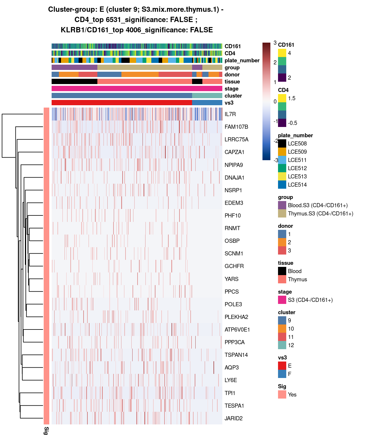
Figure 11: Heatmap of log-expression values in each sample for the top uniquely upregulated marker genes. Each column is a sample, each row a gene. Colours are capped at -3 and 3 to preserve dynamic range. Ranking of CD4 and CD161/KLRB1 from top of the DGE list sorted in ascending order of FDR and their statistical significance (TRUE = FDR < 0.05) are provided in the title.

Show code

##########################################################
# look at cluster-group F / cluster 12 (i.e. S3.mix.more.thymus.4.center)
chosen <- "F"
F_uniquely_up <- vs3_uniquely_up[[chosen]]

# add description for the chosen cluster-group
x <- "(cluster 12; S3.mix.more.thymus.4.center)"

# look only at protein coding gene (pcg)
# NOTE: not suggest to narrow down into pcg as it remove all significant candidates (FDR << 0.05) !
# F_uniquely_up_pcg <- F_uniquely_up[intersect(protein_coding_gene_set, rownames(F_uniquely_up)), ]

# get rid of noise (i.e. pseudo, ribo, mito, sex) that collaborator not interested in
F_uniquely_up_noiseR <- F_uniquely_up[setdiff(rownames(F_uniquely_up), c(pseudogene_set, mito_set, ribo_set, sex_set)), ]

# see if key marker, "CD4 and/or ""KLRB1/CD161"", contain in the DE list + if it is "significant (i.e FDR <0.05)
y <- c("CD4",
       which(rownames(F_uniquely_up_noiseR) %in% "CD4"),
       F_uniquely_up_noiseR[which(rownames(F_uniquely_up_noiseR) %in% "CD4"), ]$FDR < 0.05)
z <- c("KLRB1/CD161",
       which(rownames(F_uniquely_up_noiseR) %in% "KLRB1"),
       F_uniquely_up_noiseR[which(rownames(F_uniquely_up_noiseR) %in% "KLRB1"), ]$FDR < 0.05)

# top25 only + gene-of-interest
best_set <- F_uniquely_up_noiseR[1:25, ]

Show code

# heatmap
plotHeatmap(
  cp,
  features = rownames(best_set),
  columns = order(
    cp$vs3,
    cp$cluster,
    cp$stage,
    cp$tissue,
    cp$donor,
    cp$group,
    cp$plate_number,
    cp$CD4,
    cp$CD161),
  colour_columns_by = c(
    "vs3",
    "cluster",
    "stage",
    "tissue",
    "donor",
    "group",
    "plate_number",
    "CD4",
    "CD161"),
  cluster_cols = FALSE,
  center = TRUE,
  symmetric = TRUE,
  zlim = c(-3, 3),
  show_colnames = FALSE,
  annotation_row = data.frame(
    Sig = factor(
      ifelse(best_set[, "FDR"] < 0.05, "Yes", "No"),
      # TODO: temp trick to deal with the row-colouring problem
      # levels = c("Yes", "No")),
      levels = c("Yes")),
    row.names = rownames(best_set)),
  main = paste0("Cluster-group: ", chosen, " ", x, " - \n",
                y[1], "_top ", y[2], "_significance: ", y[3], " ; \n",
                z[1], "_top ", z[2], "_significance: ", z[3]),
  column_annotation_colors = list(
    # Sig = c("Yes" = "red", "No" = "lightgrey"),
    vs3 = vs3_colours,
    cluster = cluster_colours,
    stage = stage_colours,
    tissue = tissue_colours,
    donor = donor_colours,
    group = group_colours,
    plate_number = plate_number_colours),
  color = hcl.colors(101, "Blue-Red 3"),
  fontsize = 7)

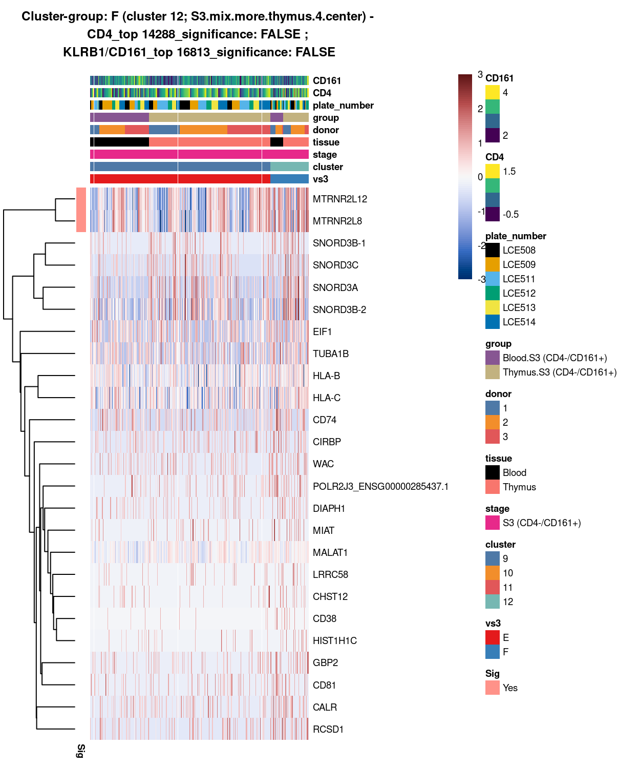
Figure 12: Heatmap of log-expression values in each sample for the top uniquely upregulated marker genes. Each column is a sample, each row a gene. Colours are capped at -3 and 3 to preserve dynamic range. Ranking of CD4 and CD161/KLRB1 from top of the DGE list sorted in ascending order of FDR and their statistical significance (TRUE = FDR < 0.05) are provided in the title.

DGE lists of these comparisons are available in output/marker_genes/S3_only/uniquely_up/cluster_9_vs_12/.

SUMMARY: 9 vs 12 (E vs F)

• cluster 9 (S3.mix.more.thymus.1 >>> cluster 9 does show a number of cells more frequently expressed with lots of markers (not associated with tissue)
• cluster 12 (S3.mix.more.thymus.4.center >>> beside the two mitochondrial genes (i.e. most likely be noise) no sig marker found, though, visually, there seems like some
• COMMENT: gene expression pattern of cluster 12 should be similar to cluster 9; whilst cluster 9 does show a number of genes up-regulated in cluster 9, but not in cluster 12; needed to keep them apart

cluster_10_vs_cluster_11

Show code

#########
# G vs H
#########

##########################################################################################
# cluster 10 (i.e. S3.mix.more.thymus.2) vs cluster 11 (i.e. S3.mix.more.thymus.3)

# checkpoint
cp <- sce
# exclude cells of uninterested cluster from cp
cp <- cp[, cp$cluster == "10" | cp$cluster == "11"]
colData(cp) <- droplevels(colData(cp))

# classify cluster-group for comparison
cp$vs4 <- factor(ifelse(cp$cluster == 10, "G", "H"))

# set vs colours
vs4_colours <- setNames(
  palette.colors(nlevels(cp$vs4), "Set1"),
  levels(cp$vs4))
cp$colours$vs4_colours <- vs4_colours[cp$vs4]

# find unique DE ./. cluster-groups
vs4_uniquely_up <- findMarkers(
  cp,
  groups = cp$vs4,
  block = cp$block,
  pval.type = "all",
  direction = "up")

# export DGE lists
saveRDS(
  vs4_uniquely_up,
  here("data", "marker_genes", "S3_only", "C094_Pellicci.uniquely_up.cluster_10_vs_11.rds"),
  compress = "xz")

dir.create(here("output", "marker_genes", "S3_only", "uniquely_up", "cluster_10_vs_11"), recursive = TRUE)

vs_pair <- c("10", "11")

message("Writing 'uniquely_up (cluster_10_vs_11)' marker genes to file.")
for (n in names(vs4_uniquely_up)) {
  message(n)
  gzout <- gzfile(
    description = here(
      "output",
      "marker_genes",
      "S3_only",
      "uniquely_up",
      "cluster_10_vs_11",
      paste0("cluster_",
             vs_pair[which(names(vs4_uniquely_up) %in% n)],
             "_vs_",
             vs_pair[-which(names(vs4_uniquely_up) %in% n)][1],
             ".uniquely_up.csv.gz")),
    open = "wb")
  write.table(
    x = vs4_uniquely_up[[n]] %>%
      as.data.frame() %>%
      tibble::rownames_to_column("gene_ID"),
    file = gzout,
    sep = ",",
    quote = FALSE,
    row.names = FALSE,
    col.names = TRUE)
  close(gzout)
}

Show code

###############################################################
# look at cluster-group G / cluster 10 (i.e. S3.mix.more.thymus.2)
chosen <- "G"
G_uniquely_up <- vs4_uniquely_up[[chosen]]

# add description for the chosen cluster-group
x <- "(cluster 10; S3.mix.more.thymus.2)"

# look only at protein coding gene (pcg)
# NOTE: not suggest to narrow down into pcg as it remove all significant candidates (FDR << 0.05) !
# G_uniquely_up_pcg <- G_uniquely_up[intersect(protein_coding_gene_set, rownames(G_uniquely_up)), ]

# get rid of noise (i.e. pseudo, ribo, mito, sex) that collaborator not interested in
G_uniquely_up_noiseR <- G_uniquely_up[setdiff(rownames(G_uniquely_up), c(pseudogene_set, mito_set, ribo_set, sex_set)), ]

# see if key marker, "CD4 and/or ""KLRB1/CD161"", contain in the DE list + if it is "significant (i.e FDR <0.05)
y <- c("CD4",
       which(rownames(G_uniquely_up_noiseR) %in% "CD4"),
       G_uniquely_up_noiseR[which(rownames(G_uniquely_up_noiseR) %in% "CD4"), ]$FDR < 0.05)
z <- c("KLRB1/CD161",
       which(rownames(G_uniquely_up_noiseR) %in% "KLRB1"),
       G_uniquely_up_noiseR[which(rownames(G_uniquely_up_noiseR) %in% "KLRB1"), ]$FDR < 0.05)

# top25 only + gene-of-interest
best_set <- G_uniquely_up_noiseR[1:25, ]

Show code

# heatmap
plotHeatmap(
  cp,
  features = rownames(best_set),
  columns = order(
    cp$vs4,
    cp$cluster,
    cp$stage,
    cp$tissue,
    cp$donor,
    cp$group,
    cp$plate_number,
    cp$CD4,
    cp$CD161),
  colour_columns_by = c(
    "vs4",
    "cluster",
    "stage",
    "tissue",
    "donor",
    "group",
    "plate_number",
    "CD4",
    "CD161"),
  cluster_cols = FALSE,
  center = TRUE,
  symmetric = TRUE,
  zlim = c(-3, 3),
  show_colnames = FALSE,
  annotation_row = data.frame(
    Sig = factor(
      ifelse(best_set[, "FDR"] < 0.05, "Yes", "No"),
      # TODO: temp trick to deal with the row-colouring problem
      # levels = c("Yes", "No")),
      levels = c("Yes")),
    row.names = rownames(best_set)),
  main = paste0("Cluster-group: ", chosen, " ", x, " - \n",
                y[1], "_top ", y[2], "_significance: ", y[3], " ; \n",
                z[1], "_top ", z[2], "_significance: ", z[3]),
  column_annotation_colors = list(
    # Sig = c("Yes" = "red", "No" = "lightgrey"),
    vs4 = vs4_colours,
    cluster = cluster_colours,
    stage = stage_colours,
    tissue = tissue_colours,
    donor = donor_colours,
    group = group_colours,
    plate_number = plate_number_colours),
  color = hcl.colors(101, "Blue-Red 3"),
  fontsize = 7)

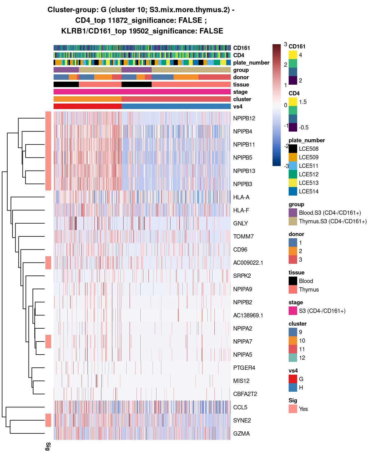
Figure 13: Heatmap of log-expression values in each sample for the top uniquely upregulated marker genes. Each column is a sample, each row a gene. Colours are capped at -3 and 3 to preserve dynamic range. Ranking of CD4 and CD161/KLRB1 from top of the DGE list sorted in ascending order of FDR and their statistical significance (TRUE = FDR < 0.05) are provided in the title.

Show code

##########################################################
# look at cluster-group H / cluster 11 (i.e. S3.mix.more.thymus.3)
chosen <- "H"
H_uniquely_up <- vs4_uniquely_up[[chosen]]

# add description for the chosen cluster-group
x <- "(cluster 11; S3.mix.more.thymus.3)"

# look only at protein coding gene (pcg)
# NOTE: not suggest to narrow down into pcg as it remove all significant candidates (FDR << 0.05) !
# H_uniquely_up_pcg <- H_uniquely_up[intersect(protein_coding_gene_set, rownames(H_uniquely_up)), ]

# get rid of noise (i.e. pseudo, ribo, mito, sex) that collaborator not interested in
H_uniquely_up_noiseR <- H_uniquely_up[setdiff(rownames(H_uniquely_up), c(pseudogene_set, mito_set, ribo_set, sex_set)), ]

# see if key marker, "CD4 and/or ""KLRB1/CD161"", contain in the DE list + if it is "significant (i.e FDR <0.05)
y <- c("CD4",
       which(rownames(H_uniquely_up_noiseR) %in% "CD4"),
       H_uniquely_up_noiseR[which(rownames(H_uniquely_up_noiseR) %in% "CD4"), ]$FDR < 0.05)
z <- c("KLRB1/CD161",
       which(rownames(H_uniquely_up_noiseR) %in% "KLRB1"),
       H_uniquely_up_noiseR[which(rownames(H_uniquely_up_noiseR) %in% "KLRB1"), ]$FDR < 0.05)

# top25 only + gene-of-interest
best_set <- H_uniquely_up_noiseR[1:25, ]

Show code

# heatmap
plotHeatmap(
  cp,
  features = rownames(best_set),
  columns = order(
    cp$vs4,
    cp$cluster,
    cp$stage,
    cp$tissue,
    cp$donor,
    cp$group,
    cp$plate_number,
    cp$CD4,
    cp$CD161),
  colour_columns_by = c(
    "vs4",
    "cluster",
    "stage",
    "tissue",
    "donor",
    "group",
    "plate_number",
    "CD4",
    "CD161"),
  cluster_cols = FALSE,
  center = TRUE,
  symmetric = TRUE,
  zlim = c(-3, 3),
  show_colnames = FALSE,
  # annotation_row = data.frame(
  #   Sig = factor(
  #     ifelse(best_set[, "FDR"] < 0.05, "Yes", "No"),
  #     # TODO: temp trick to deal with the row-colouring problem
  #     # levels = c("Yes", "No")),
  #     levels = c("Yes")),
  #   row.names = rownames(best_set)),
  main = paste0("Cluster-group: ", chosen, " ", x, " - \n",
                y[1], "_top ", y[2], "_significance: ", y[3], " ; \n",
                z[1], "_top ", z[2], "_significance: ", z[3]),
  column_annotation_colors = list(
    # Sig = c("Yes" = "red", "No" = "lightgrey"),
    vs4 = vs4_colours,
    cluster = cluster_colours,
    stage = stage_colours,
    tissue = tissue_colours,
    donor = donor_colours,
    group = group_colours,
    plate_number = plate_number_colours),
  color = hcl.colors(101, "Blue-Red 3"),
  fontsize = 7)

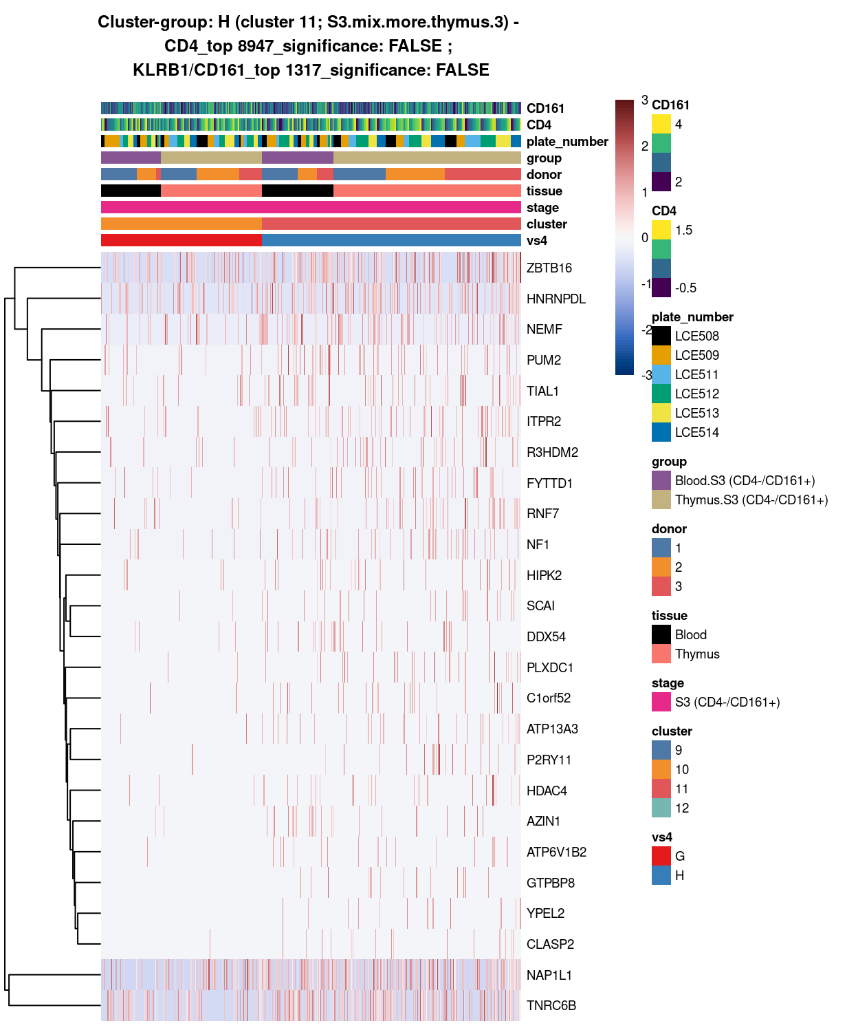
Figure 14: Heatmap of log-expression values in each sample for the top uniquely upregulated marker genes. Each column is a sample, each row a gene. Colours are capped at -3 and 3 to preserve dynamic range. Ranking of CD4 and CD161/KLRB1 from top of the DGE list sorted in ascending order of FDR and their statistical significance (TRUE = FDR < 0.05) are provided in the title.

DGE lists of these comparisons are available in output/marker_genes/S3_only/uniquely_up/cluster_10_vs_11/.

SUMMARY: 10 vs 11 (G vs H)

• cluster 10 (S3.mix.more.thymus.2 >>> besides NPIPB, SYNE2 and AC009022.9 are clear markers
• cluster 11 (S3.mix.more.thymus.3 >>> no statistically significant markers
• COMMENT: SYNE2 and AC009022.1 (and maybe NPIPB) may driven cluster 10 from 11

cluster_10_vs_cluster_12

Show code

#########
# I vs J
#########

##########################################################################################
# cluster 10 (i.e. S3.mix.more.thymus.2) vs cluster 12 (i.e. S3.mix.more.thymus.4.center)

# checkpoint
cp <- sce
# exclude cells of uninterested cluster from cp
cp <- cp[, cp$cluster == "10" | cp$cluster == "12"]
colData(cp) <- droplevels(colData(cp))

# classify cluster-group for comparison
cp$vs5 <- factor(ifelse(cp$cluster == 10, "I", "J"))

# set vs colours
vs5_colours <- setNames(
  palette.colors(nlevels(cp$vs5), "Set1"),
  levels(cp$vs5))
cp$colours$vs5_colours <- vs5_colours[cp$vs5]

# find unique DE ./. cluster-groups
vs5_uniquely_up <- findMarkers(
  cp,
  groups = cp$vs5,
  block = cp$block,
  pval.type = "all",
  direction = "up")

# export DGE lists
saveRDS(
  vs5_uniquely_up,
  here("data", "marker_genes", "S3_only", "C094_Pellicci.uniquely_up.cluster_10_vs_12.rds"),
  compress = "xz")

dir.create(here("output", "marker_genes", "S3_only", "uniquely_up", "cluster_10_vs_12"), recursive = TRUE)

vs_pair <- c("10", "12")

message("Writing 'uniquely_up (cluster_10_vs_12)' marker genes to file.")
for (n in names(vs5_uniquely_up)) {
  message(n)
  gzout <- gzfile(
    description = here(
      "output",
      "marker_genes",
      "S3_only",
      "uniquely_up",
      "cluster_10_vs_12",
      paste0("cluster_",
             vs_pair[which(names(vs5_uniquely_up) %in% n)],
             "_vs_",
             vs_pair[-which(names(vs5_uniquely_up) %in% n)][1],
             ".uniquely_up.csv.gz")),
    open = "wb")
  write.table(
    x = vs5_uniquely_up[[n]] %>%
      as.data.frame() %>%
      tibble::rownames_to_column("gene_ID"),
    file = gzout,
    sep = ",",
    quote = FALSE,
    row.names = FALSE,
    col.names = TRUE)
  close(gzout)
}

Show code

###############################################################
# look at cluster-group I / cluster 10 (i.e. S3.mix.more.thymus.2)
chosen <- "I"
I_uniquely_up <- vs5_uniquely_up[[chosen]]

# add description for the chosen cluster-group
x <- "(cluster 10; S3.mix.more.thymus.2)"

# look only at protein coding gene (pcg)
# NOTE: not suggest to narrow down into pcg as it remove all significant candidates (FDR << 0.05) !
# I_uniquely_up_pcg <- I_uniquely_up[intersect(protein_coding_gene_set, rownames(I_uniquely_up)), ]

# get rid of noise (i.e. pseudo, ribo, mito, sex) that collaborator not interested in
I_uniquely_up_noiseR <- I_uniquely_up[setdiff(rownames(I_uniquely_up), c(pseudogene_set, mito_set, ribo_set, sex_set)), ]

# see if key marker, "CD4 and/or ""KLRB1/CD161"", contain in the DE list + if it is "significant (i.e FDR <0.05)
y <- c("CD4",
       which(rownames(I_uniquely_up_noiseR) %in% "CD4"),
       I_uniquely_up_noiseR[which(rownames(I_uniquely_up_noiseR) %in% "CD4"), ]$FDR < 0.05)
z <- c("KLRB1/CD161",
       which(rownames(I_uniquely_up_noiseR) %in% "KLRB1"),
       I_uniquely_up_noiseR[which(rownames(I_uniquely_up_noiseR) %in% "KLRB1"), ]$FDR < 0.05)

# top25 only + gene-of-interest
best_set <- I_uniquely_up_noiseR[1:25, ]

Show code

# heatmap
plotHeatmap(
  cp,
  features = rownames(best_set),
  columns = order(
    cp$vs5,
    cp$cluster,
    cp$stage,
    cp$tissue,
    cp$donor,
    cp$group,
    cp$plate_number,
    cp$CD4,
    cp$CD161),
  colour_columns_by = c(
    "vs5",
    "cluster",
    "stage",
    "tissue",
    "donor",
    "group",
    "plate_number",
    "CD4",
    "CD161"),
  cluster_cols = FALSE,
  center = TRUE,
  symmetric = TRUE,
  zlim = c(-3, 3),
  show_colnames = FALSE,
  annotation_row = data.frame(
    Sig = factor(
      ifelse(best_set[, "FDR"] < 0.05, "Yes", "No"),
      # TODO: temp trick to deal with the row-colouring problem
      # levels = c("Yes", "No")),
      levels = c("Yes")),
    row.names = rownames(best_set)),
  main = paste0("Cluster-group: ", chosen, " ", x, " - \n",
                y[1], "_top ", y[2], "_significance: ", y[3], " ; \n",
                z[1], "_top ", z[2], "_significance: ", z[3]),
  column_annotation_colors = list(
    # Sig = c("Yes" = "red", "No" = "lightgrey"),
    vs5 = vs5_colours,
    cluster = cluster_colours,
    stage = stage_colours,
    tissue = tissue_colours,
    donor = donor_colours,
    group = group_colours,
    plate_number = plate_number_colours),
  color = hcl.colors(101, "Blue-Red 3"),
  fontsize = 7)

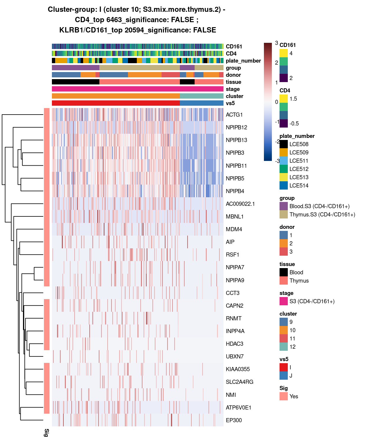
Figure 15: Heatmap of log-expression values in each sample for the top uniquely upregulated marker genes. Each column is a sample, each row a gene. Colours are capped at -3 and 3 to preserve dynamic range. Ranking of CD4 and CD161/KLRB1 from top of the DGE list sorted in ascending order of FDR and their statistical significance (TRUE = FDR < 0.05) are provided in the title.

Show code

##########################################################
# look at cluster-group J / cluster 12 (i.e. S3.mix.more.thymus.4.center)
chosen <- "J"
J_uniquely_up <- vs5_uniquely_up[[chosen]]

# add description for the chosen cluster-group
x <- "(cluster 12; S3-mix, set 4)"

# look only at protein coding gene (pcg)
# NOTE: not suggest to narrow down into pcg as it remove all significant candidates (FDR << 0.05) !
# J_uniquely_up_pcg <- J_uniquely_up[intersect(protein_coding_gene_set, rownames(J_uniquely_up)), ]

# get rid of noise (i.e. pseudo, ribo, mito, sex) that collaborator not interested in
J_uniquely_up_noiseR <- J_uniquely_up[setdiff(rownames(J_uniquely_up), c(pseudogene_set, mito_set, ribo_set, sex_set)), ]

# see if key marker, "CD4 and/or ""KLRB1/CD161"", contain in the DE list + if it is "significant (i.e FDR <0.05)
y <- c("CD4",
       which(rownames(J_uniquely_up_noiseR) %in% "CD4"),
       J_uniquely_up_noiseR[which(rownames(J_uniquely_up_noiseR) %in% "CD4"), ]$FDR < 0.05)
z <- c("KLRB1/CD161",
       which(rownames(J_uniquely_up_noiseR) %in% "KLRB1"),
       J_uniquely_up_noiseR[which(rownames(J_uniquely_up_noiseR) %in% "KLRB1"), ]$FDR < 0.05)

# top25 only + gene-of-interest
best_set <- J_uniquely_up_noiseR[1:25, ]

Show code

# heatmap
plotHeatmap(
  cp,
  features = rownames(best_set),
  columns = order(
    cp$vs5,
    cp$cluster,
    cp$stage,
    cp$tissue,
    cp$donor,
    cp$group,
    cp$plate_number,
    cp$CD4,
    cp$CD161),
  colour_columns_by = c(
    "vs5",
    "cluster",
    "stage",
    "tissue",
    "donor",
    "group",
    "plate_number",
    "CD4",
    "CD161"),
  cluster_cols = FALSE,
  center = TRUE,
  symmetric = TRUE,
  zlim = c(-3, 3),
  show_colnames = FALSE,
  # annotation_row = data.frame(
  #   Sig = factor(
  #     ifelse(best_set[, "FDR"] < 0.05, "Yes", "No"),
  #     # TODO: temp trick to deal with the row-colouring problem
  #     # levels = c("Yes", "No")),
  #     levels = c("Yes")),
  #   row.names = rownames(best_set)),
  main = paste0("Cluster-group: ", chosen, " ", x, " - \n",
                y[1], "_top ", y[2], "_significance: ", y[3], " ; \n",
                z[1], "_top ", z[2], "_significance: ", z[3]),
  column_annotation_colors = list(
    # Sig = c("Yes" = "red", "No" = "lightgrey"),
    vs5 = vs5_colours,
    cluster = cluster_colours,
    stage = stage_colours,
    tissue = tissue_colours,
    donor = donor_colours,
    group = group_colours,
    plate_number = plate_number_colours),
  color = hcl.colors(101, "Blue-Red 3"),
  fontsize = 7)

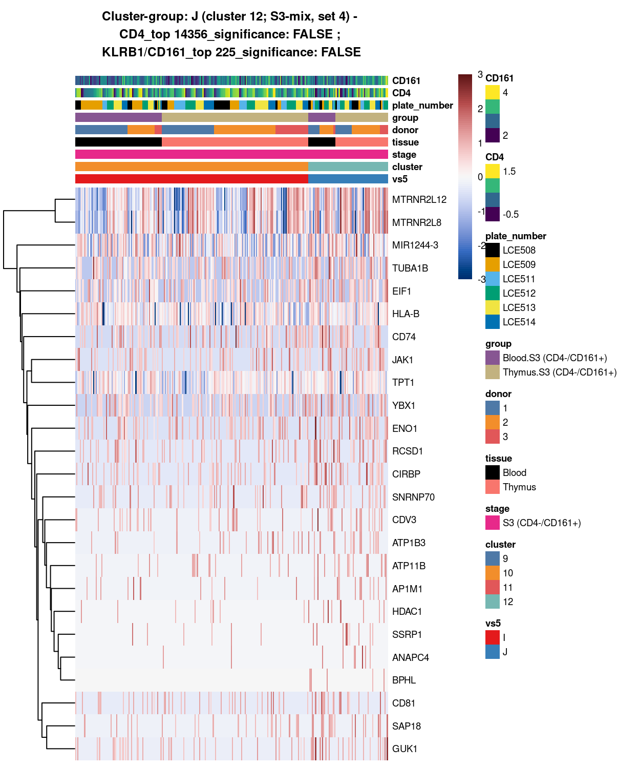
Figure 16: Heatmap of log-expression values in each sample for the top uniquely upregulated marker genes. Each column is a sample, each row a gene. Colours are capped at -3 and 3 to preserve dynamic range. Ranking of CD4 and CD161/KLRB1 from top of the DGE list sorted in ascending order of FDR and their statistical significance (TRUE = FDR < 0.05) are provided in the title.

DGE lists of these comparisons are available in output/marker_genes/S3_only/uniquely_up/cluster_10_vs_12/.

SUMMARY: 10 vs 12 (I vs J)

• cluster 10 (S3.mix.more.thymus.2 >>> besides NPIPB, got number of markers (e.g. ACTG1, MBNL1, MDM4, etc.)
• cluster 12 (S3.mix.more.thymus.4.center >>> statistically, no significant marker can be found
• COMMENT: gene like (ACTG1, MBNL1, MDM4, etc.) may drive cluster 10 away from 12 at the center

cluster_11_vs_cluster_12

Show code

#########
# K vs L
#########

##########################################################################################
# cluster 11 (i.e. S3.mix.more.thymus.3) vs cluster 12 (i.e. S3.mix.more.thymus.4.center)

# checkpoint
cp <- sce
# exclude cells of uninterested cluster from cp
cp <- cp[, cp$cluster == "11" | cp$cluster == "12"]
colData(cp) <- droplevels(colData(cp))

# classify cluster-group for comparison
cp$vs6 <- factor(ifelse(cp$cluster == 11, "K", "L"))

# set vs colours
vs6_colours <- setNames(
  palette.colors(nlevels(cp$vs6), "Set1"),
  levels(cp$vs6))
cp$colours$vs6_colours <- vs6_colours[cp$vs6]

# find unique DE ./. cluster-groups
vs6_uniquely_up <- findMarkers(
  cp,
  groups = cp$vs6,
  block = cp$block,
  pval.type = "all",
  direction = "up")

# export DGE lists
saveRDS(
  vs6_uniquely_up,
  here("data", "marker_genes", "S3_only", "C094_Pellicci.uniquely_up.cluster_11_vs_12.rds"),
  compress = "xz")

dir.create(here("output", "marker_genes", "S3_only", "uniquely_up", "cluster_11_vs_12"), recursive = TRUE)

vs_pair <- c("3", "4")

message("Writing 'uniquely_up (cluster_11_vs_12)' marker genes to file.")
for (n in names(vs6_uniquely_up)) {
  message(n)
  gzout <- gzfile(
    description = here(
      "output",
      "marker_genes",
      "S3_only",
      "uniquely_up",
      "cluster_11_vs_12",
      paste0("cluster_",
             vs_pair[which(names(vs6_uniquely_up) %in% n)],
             "_vs_",
             vs_pair[-which(names(vs6_uniquely_up) %in% n)][1],
             ".uniquely_up.csv.gz")),
    open = "wb")
  write.table(
    x = vs6_uniquely_up[[n]] %>%
      as.data.frame() %>%
      tibble::rownames_to_column("gene_ID"),
    file = gzout,
    sep = ",",
    quote = FALSE,
    row.names = FALSE,
    col.names = TRUE)
  close(gzout)
}

Show code

###############################################################
# look at cluster-group K / cluster 11 (i.e. S3.mix.more.thymus.3)
chosen <- "K"
K_uniquely_up <- vs6_uniquely_up[[chosen]]

# add description for the chosen cluster-group
x <- "(cluster 11; S3.mix.more.thymus.3)"

# look only at protein coding gene (pcg)
# NOTE: not suggest to narrow down into pcg as it remove all significant candidates (FDR << 0.05) !
# K_uniquely_up_pcg <- K_uniquely_up[intersect(protein_coding_gene_set, rownames(K_uniquely_up)), ]

# get rid of noise (i.e. pseudo, ribo, mito, sex) that collaborator not interested in
K_uniquely_up_noiseR <- K_uniquely_up[setdiff(rownames(K_uniquely_up), c(pseudogene_set, mito_set, ribo_set, sex_set)), ]

# see if key marker, "CD4 and/or ""KLRB1/CD161"", contain in the DE list + if it is "significant (i.e FDR <0.05)
y <- c("CD4",
       which(rownames(K_uniquely_up_noiseR) %in% "CD4"),
       K_uniquely_up_noiseR[which(rownames(K_uniquely_up_noiseR) %in% "CD4"), ]$FDR < 0.05)
z <- c("KLRB1/CD161",
       which(rownames(K_uniquely_up_noiseR) %in% "KLRB1"),
       K_uniquely_up_noiseR[which(rownames(K_uniquely_up_noiseR) %in% "KLRB1"), ]$FDR < 0.05)

# top25 only + gene-of-interest
best_set <- K_uniquely_up_noiseR[1:25, ]

Show code

# heatmap
plotHeatmap(
  cp,
  features = rownames(best_set),
  columns = order(
    cp$vs6,
    cp$cluster,
    cp$stage,
    cp$tissue,
    cp$donor,
    cp$group,
    cp$plate_number,
    cp$CD4,
    cp$CD161),
  colour_columns_by = c(
    "vs6",
    "cluster",
    "stage",
    "tissue",
    "donor",
    "group",
    "plate_number",
    "CD4",
    "CD161"),
  cluster_cols = FALSE,
  center = TRUE,
  symmetric = TRUE,
  zlim = c(-3, 3),
  show_colnames = FALSE,
  annotation_row = data.frame(
    Sig = factor(
      ifelse(best_set[, "FDR"] < 0.05, "Yes", "No"),
      # TODO: temp trick to deal with the row-colouring problem
      # levels = c("Yes", "No")),
      levels = c("Yes")),
    row.names = rownames(best_set)),
  main = paste0("Cluster-group: ", chosen, " ", x, " - \n",
                y[1], "_top ", y[2], "_significance: ", y[3], " ; \n",
                z[1], "_top ", z[2], "_significance: ", z[3]),
  column_annotation_colors = list(
    # Sig = c("Yes" = "red", "No" = "lightgrey"),
    vs6 = vs6_colours,
    cluster = cluster_colours,
    stage = stage_colours,
    tissue = tissue_colours,
    donor = donor_colours,
    group = group_colours,
    plate_number = plate_number_colours),
  color = hcl.colors(101, "Blue-Red 3"),
  fontsize = 7)

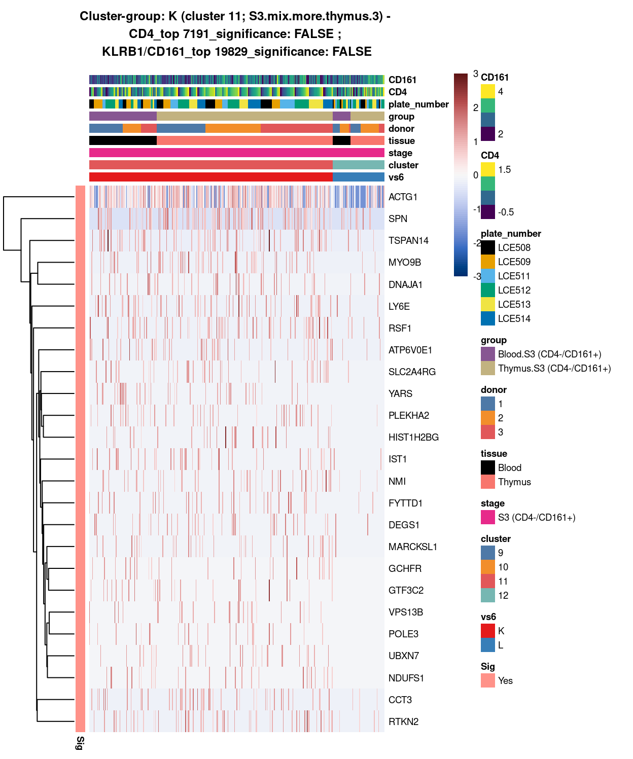
Figure 17: Heatmap of log-expression values in each sample for the top uniquely upregulated marker genes. Each column is a sample, each row a gene. Colours are capped at -3 and 3 to preserve dynamic range. Ranking of CD4 and CD161/KLRB1 from top of the DGE list sorted in ascending order of FDR and their statistical significance (TRUE = FDR < 0.05) are provided in the title.

Show code

##########################################################
# look at cluster-group L / cluster 12 (i.e. S3.mix.more.thymus.4.center)
chosen <- "L"
L_uniquely_up <- vs6_uniquely_up[[chosen]]

# add description for the chosen cluster-group
x <- "(cluster 12; S3.mix.more.thymus.4.center)"

# look only at protein coding gene (pcg)
# NOTE: not suggest to narrow down into pcg as it remove all significant candidates (FDR << 0.05) !
# L_uniquely_up_pcg <- L_uniquely_up[intersect(protein_coding_gene_set, rownames(L_uniquely_up)), ]

# get rid of noise (i.e. pseudo, ribo, mito, sex) that collaborator not interested in
L_uniquely_up_noiseR <- L_uniquely_up[setdiff(rownames(L_uniquely_up), c(pseudogene_set, mito_set, ribo_set, sex_set)), ]

# see if key marker, "CD4 and/or ""KLRB1/CD161"", contain in the DE list + if it is "significant (i.e FDR <0.05)
y <- c("CD4",
       which(rownames(L_uniquely_up_noiseR) %in% "CD4"),
       L_uniquely_up_noiseR[which(rownames(L_uniquely_up_noiseR) %in% "CD4"), ]$FDR < 0.05)
z <- c("KLRB1/CD161",
       which(rownames(L_uniquely_up_noiseR) %in% "KLRB1"),
       L_uniquely_up_noiseR[which(rownames(L_uniquely_up_noiseR) %in% "KLRB1"), ]$FDR < 0.05)

# top25 only + gene-of-interest
best_set <- L_uniquely_up_noiseR[1:25, ]

Show code

# heatmap
plotHeatmap(
  cp,
  features = rownames(best_set),
  columns = order(
    cp$vs6,
    cp$cluster,
    cp$stage,
    cp$tissue,
    cp$donor,
    cp$group,
    cp$plate_number,
    cp$CD4,
    cp$CD161),
  colour_columns_by = c(
    "vs6",
    "cluster",
    "stage",
    "tissue",
    "donor",
    "group",
    "plate_number",
    "CD4",
    "CD161"),
  cluster_cols = FALSE,
  center = TRUE,
  symmetric = TRUE,
  zlim = c(-3, 3),
  show_colnames = FALSE,
  # annotation_row = data.frame(
  #   Sig = factor(
  #     ifelse(best_set[, "FDR"] < 0.05, "Yes", "No"),
  #     # TODO: temp trick to deal with the row-colouring problem
  #     # levels = c("Yes", "No")),
  #     levels = c("Yes")),
  #   row.names = rownames(best_set)),
  main = paste0("Cluster-group: ", chosen, " ", x, " - \n",
                y[1], "_top ", y[2], "_significance: ", y[3], " ; \n",
                z[1], "_top ", z[2], "_significance: ", z[3]),
  column_annotation_colors = list(
    # Sig = c("Yes" = "red", "No" = "lightgrey"),
    vs6 = vs6_colours,
    cluster = cluster_colours,
    stage = stage_colours,
    tissue = tissue_colours,
    donor = donor_colours,
    group = group_colours,
    plate_number = plate_number_colours),
  color = hcl.colors(101, "Blue-Red 3"),
  fontsize = 7)

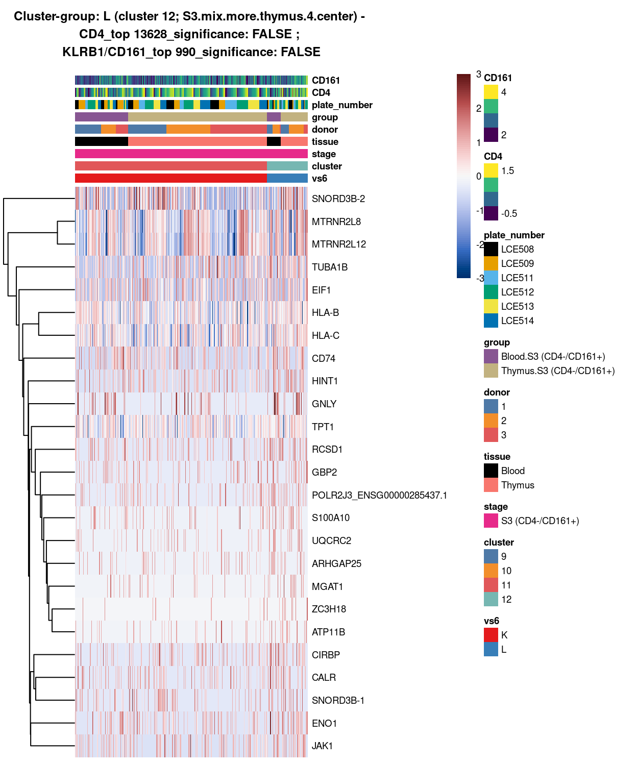
Figure 18: Heatmap of log-expression values in each sample for the top uniquely upregulated marker genes. Each column is a sample, each row a gene. Colours are capped at -3 and 3 to preserve dynamic range. Ranking of CD4 and CD161/KLRB1 from top of the DGE list sorted in ascending order of FDR and their statistical significance (TRUE = FDR < 0.05) are provided in the title.

DGE lists of these comparisons are available in output/marker_genes/S3_only/uniquely_up/cluster_11_vs_12/.

SUMMARY: 11 vs 12 (K vs L)

• cluster 11 (S3.mix.more.thymus.3 >>> got lots of genes statistically sig express in cluster 11 only, e.g. ACTG1, IST1, CCT3, etc.
• cluster 12 (S3.mix.more.thymus.4.center >>> no statistically significant markers found
• COMMENT: cluster 11 got number of unique markers (e.g. e.g. ACTG1, IST1, CCT3, etc.) and drove cluster 11 from 12

cluster_9_10_vs_cluster_11

Show code

#########
# M vs N
#########

##########################################################################################
# cluster 9 (i.e. S3.mix.more.thymus.1) vs cluster 10 (i.e. S3.mix.more.thymus.2)

# checkpoint
cp <- sce
# exclude cells of uninterested cluster from cp
cp <- cp[, cp$cluster == "9" | cp$cluster == "10" | cp$cluster == "11"]
colData(cp) <- droplevels(colData(cp))

# classify cluster-group for comparison
cp$vs7 <- factor(ifelse(cp$cluster == 9 | cp$cluster == 10, "M", "N"))

# set vs colours
vs7_colours <- setNames(
  palette.colors(nlevels(cp$vs7), "Set1"),
  levels(cp$vs7))
cp$colours$vs7_colours <- vs7_colours[cp$vs7]

# find unique DE ./. cluster-groups
vs7_uniquely_up <- findMarkers(
  cp,
  groups = cp$vs7,
  block = cp$block,
  pval.type = "all",
  direction = "up")

# export DGE lists
saveRDS(
  vs7_uniquely_up,
  here("data", "marker_genes", "S3_only", "C094_Pellicci.uniquely_up.cluster_9_10_vs_11.rds"),
  compress = "xz")

dir.create(here("output", "marker_genes", "S3_only", "uniquely_up", "cluster_9_10_vs_11"), recursive = TRUE)

vs_pair <- c("9_10", "11")

message("Writing 'uniquely_up (cluster_9_10_vs_11)' marker genes to file.")
for (n in names(vs7_uniquely_up)) {
  message(n)
  gzout <- gzfile(
    description = here(
      "output",
      "marker_genes",
      "S3_only",
      "uniquely_up",
      "cluster_9_10_vs_11",
      paste0("cluster_",
             vs_pair[which(names(vs7_uniquely_up) %in% n)],
             "_vs_",
             vs_pair[-which(names(vs7_uniquely_up) %in% n)][1],
             ".uniquely_up.csv.gz")),
    open = "wb")
  write.table(
    x = vs7_uniquely_up[[n]] %>%
      as.data.frame() %>%
      tibble::rownames_to_column("gene_ID"),
    file = gzout,
    sep = ",",
    quote = FALSE,
    row.names = FALSE,
    col.names = TRUE)
  close(gzout)
}

Show code

###############################################################
# look at cluster-group M / cluster 9_10 (i.e. S3.mix.more.thymus.1.and.2)
chosen <- "M"
M_uniquely_up <- vs7_uniquely_up[[chosen]]

# add description for the chosen cluster-group
x <- "(cluster 9_10; S3.mix.more.thymus.1.and.2)"

# look only at protein coding gene (pcg)
# NOTE: not suggest to narrow down into pcg as it remove all significant candidates (FDR << 0.05) !
# M_uniquely_up_pcg <- M_uniquely_up[intersect(protein_coding_gene_set, rownames(M_uniquely_up)), ]

# get rid of noise (i.e. pseudo, ribo, mito, sex) that collaborator not interested in
M_uniquely_up_noiseR <- M_uniquely_up[setdiff(rownames(M_uniquely_up), c(pseudogene_set, mito_set, ribo_set, sex_set)), ]

# see if key marker, "CD4 and/or ""KLRB1/CD161"", contain in the DE list + if it is "significant (i.e FDR <0.05)
y <- c("CD4",
       which(rownames(M_uniquely_up_noiseR) %in% "CD4"),
       M_uniquely_up_noiseR[which(rownames(M_uniquely_up_noiseR) %in% "CD4"), ]$FDR < 0.05)
z <- c("KLRB1/CD161",
       which(rownames(M_uniquely_up_noiseR) %in% "KLRB1"),
       M_uniquely_up_noiseR[which(rownames(M_uniquely_up_noiseR) %in% "KLRB1"), ]$FDR < 0.05)

# top25 only + gene-of-interest
best_set <- M_uniquely_up_noiseR[1:25, ]

Show code

# heatmap
plotHeatmap(
  cp,
  features = rownames(best_set),
  columns = order(
    cp$vs7,
    cp$cluster,
    cp$stage,
    cp$tissue,
    cp$donor,
    cp$group,
    cp$plate_number,
    cp$CD4,
    cp$CD161),
  colour_columns_by = c(
    "vs7",
    "cluster",
    "stage",
    "tissue",
    "donor",
    "group",
    "plate_number",
    "CD4",
    "CD161"),
  cluster_cols = FALSE,
  center = TRUE,
  symmetric = TRUE,
  zlim = c(-3, 3),
  show_colnames = FALSE,
  # annotation_row = data.frame(
  #   Sig = factor(
  #     ifelse(best_set[, "FDR"] < 0.05, "Yes", "No"),
  #     # TODO: temp trick to deal with the row-colouring problem
  #     # levels = c("Yes", "No")),
  #     levels = c("Yes")),
  #   row.names = rownames(best_set)),
  main = paste0("Cluster-group: ", chosen, " ", x, " - \n",
                y[1], "_top ", y[2], "_significance: ", y[3], " ; \n",
                z[1], "_top ", z[2], "_significance: ", z[3]),
  column_annotation_colors = list(
    # Sig = c("Yes" = "red", "No" = "lightgrey"),
    vs7 = vs7_colours,
    cluster = cluster_colours,
    stage = stage_colours,
    tissue = tissue_colours,
    donor = donor_colours,
    group = group_colours,
    plate_number = plate_number_colours),
  color = hcl.colors(101, "Blue-Red 3"),
  fontsize = 7)

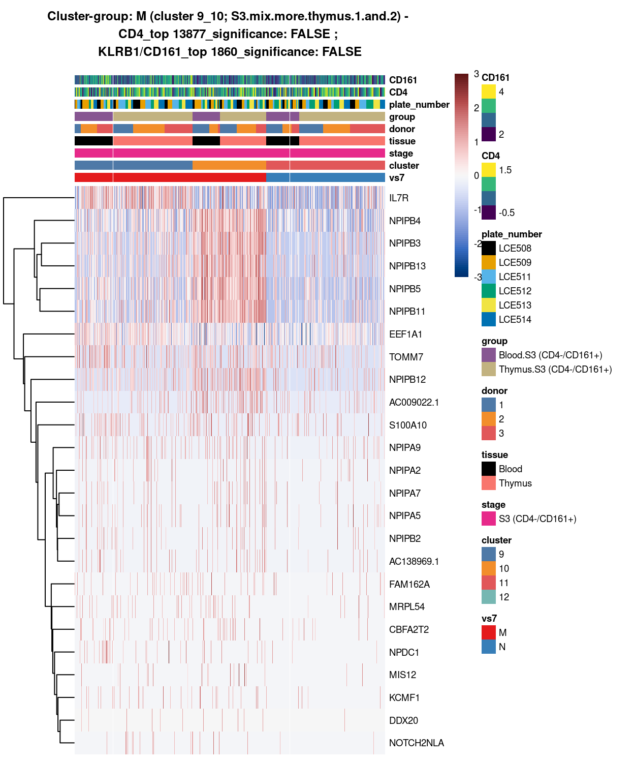
(#fig:heat-uniquely-up-logExp-cluster-9_10-vs-11)Heatmap of log-expression values in each sample for the top uniquely upregulated marker genes. Each column is a sample, each row a gene. Colours are capped at -3 and 3 to preserve dynamic range. Ranking of CD4 and CD161/KLRB1 from top of the DGE list sorted in ascending order of FDR and their statistical significance (TRUE = FDR < 0.05) are provided in the title.

Show code

##########################################################
# look at cluster-group N / cluster 11 (i.e. S3.mix.more.thymus.3)
chosen <- "N"
N_uniquely_up <- vs7_uniquely_up[[chosen]]

# add description for the chosen cluster-group
x <- "(cluster 11; S3.mix.more.thymus.3)"

# look only at protein coding gene (pcg)
# NOTE: not suggest to narrow down into pcg as it remove all significant candidates (FDR << 0.05) !
# N_uniquely_up_pcg <- N_uniquely_up[intersect(protein_coding_gene_set, rownames(N_uniquely_up)), ]

# get rid of noise (i.e. pseudo, ribo, mito, sex) that collaborator not interested in
N_uniquely_up_noiseR <- N_uniquely_up[setdiff(rownames(N_uniquely_up), c(pseudogene_set, mito_set, ribo_set, sex_set)), ]

# see if key marker, "CD4 and/or ""KLRB1/CD161"", contain in the DE list + if it is "significant (i.e FDR <0.05)
y <- c("CD4",
       which(rownames(N_uniquely_up_noiseR) %in% "CD4"),
       N_uniquely_up_noiseR[which(rownames(N_uniquely_up_noiseR) %in% "CD4"), ]$FDR < 0.05)
z <- c("KLRB1/CD161",
       which(rownames(N_uniquely_up_noiseR) %in% "KLRB1"),
       N_uniquely_up_noiseR[which(rownames(N_uniquely_up_noiseR) %in% "KLRB1"), ]$FDR < 0.05)

# top25 only + gene-of-interest
best_set <- N_uniquely_up_noiseR[1:25, ]

Show code

# heatmap
plotHeatmap(
  cp,
  features = rownames(best_set),
  columns = order(
    cp$vs7,
    cp$cluster,
    cp$stage,
    cp$tissue,
    cp$donor,
    cp$group,
    cp$plate_number,
    cp$CD4,
    cp$CD161),
  colour_columns_by = c(
    "vs7",
    "cluster",
    "stage",
    "tissue",
    "donor",
    "group",
    "plate_number",
    "CD4",
    "CD161"),
  cluster_cols = FALSE,
  center = TRUE,
  symmetric = TRUE,
  zlim = c(-3, 3),
  show_colnames = FALSE,
  # annotation_row = data.frame(
  #   Sig = factor(
  #     ifelse(best_set[, "FDR"] < 0.05, "Yes", "No"),
  #     # TODO: temp trick to deal with the row-colouring problem
  #     # levels = c("Yes", "No")),
  #     levels = c("Yes")),
  # row.names = rownames(best_set)),
  main = paste0("Cluster-group: ", chosen, " ", x, " - \n",
                y[1], "_top ", y[2], "_significance: ", y[3], " ; \n",
                z[1], "_top ", z[2], "_significance: ", z[3]),
  column_annotation_colors = list(
    # Sig = c("Yes" = "red", "No" = "lightgrey"),
    vs7 = vs7_colours,
    cluster = cluster_colours,
    stage = stage_colours,
    tissue = tissue_colours,
    donor = donor_colours,
    group = group_colours,
    plate_number = plate_number_colours),
  color = hcl.colors(101, "Blue-Red 3"),
  fontsize = 7)

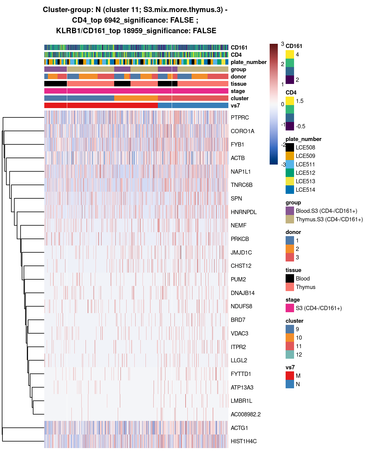
(#fig:heat-uniquely-up-logExp-cluster-11-vs-9_10)Heatmap of log-expression values in each sample for the top uniquely upregulated marker genes. Each column is a sample, each row a gene. Colours are capped at -3 and 3 to preserve dynamic range. Ranking of CD4 and CD161/KLRB1 from top of the DGE list sorted in ascending order of FDR and their statistical significance (TRUE = FDR < 0.05) are provided in the title.

DGE lists of these comparisons are available in output/marker_genes/S3_only/uniquely_up/cluster_9_10_vs_11/.

SUMMARY: 9_10 vs 11 (M vs N)

• cluster 1_2 (S3.mix.more.thymus.1.and.2 >>> statistically no significant marker could be found
• cluster 11 (S3.mix.more.thymus.3 >>> statistically no significant marker could be found
• COMMENT: could it be the case that when cluster 9 and 10 are too different; when compare something that is “internally different” with another cluster would decrease the statistical power (as both 9_vs_11 and 10_vs_11 are proven to be different)?

cluster_10_11_vs_cluster_9

Show code

#########
# O vs P
#########

##########################################################################################
# cluster 10_11 (i.e. S3.mix.more.thymus.2.and.3) vs cluster 9 (i.e. S3.mix.more.thymus.1)

# checkpoint
cp <- sce
# exclude cells of uninterested cluster from cp
cp <- cp[, cp$cluster == "9" | cp$cluster == "10" | cp$cluster == "11"]
colData(cp) <- droplevels(colData(cp))

# classify cluster-group for comparison
cp$vs8 <- factor(ifelse(cp$cluster == 10 | cp$cluster == 11, "O", "P"))

# set vs colours
vs8_colours <- setNames(
  palette.colors(nlevels(cp$vs8), "Set1"),
  levels(cp$vs8))
cp$colours$vs8_colours <- vs8_colours[cp$vs8]

# find unique DE ./. cluster-groups
vs8_uniquely_up <- findMarkers(
  cp,
  groups = cp$vs8,
  block = cp$block,
  pval.type = "all",
  direction = "up")

# export DGE lists
saveRDS(
  vs8_uniquely_up,
  here("data", "marker_genes", "S3_only", "C094_Pellicci.uniquely_up.cluster_10_11_vs_9.rds"),
  compress = "xz")

dir.create(here("output", "marker_genes", "S3_only", "uniquely_up", "cluster_10_11_vs_9"), recursive = TRUE)

vs_pair <- c("10_11", "9")

message("Writing 'uniquely_up (cluster_10_11_vs_9)' marker genes to file.")
for (n in names(vs8_uniquely_up)) {
  message(n)
  gzout <- gzfile(
    description = here(
      "output",
      "marker_genes",
      "S3_only",
      "uniquely_up",
      "cluster_10_11_vs_9",
      paste0("cluster_",
             vs_pair[which(names(vs8_uniquely_up) %in% n)],
             "_vs_",
             vs_pair[-which(names(vs8_uniquely_up) %in% n)][1],
             ".uniquely_up.csv.gz")),
    open = "wb")
  write.table(
    x = vs8_uniquely_up[[n]] %>%
      as.data.frame() %>%
      tibble::rownames_to_column("gene_ID"),
    file = gzout,
    sep = ",",
    quote = FALSE,
    row.names = FALSE,
    col.names = TRUE)
  close(gzout)
}

Show code

###############################################################
# look at cluster-group O / cluster 10_11 (i.e. S3.mix.more.thymus.2.and.3)
chosen <- "O"
O_uniquely_up <- vs8_uniquely_up[[chosen]]

# add description for the chosen cluster-group
x <- "(cluster 10_11; S3.mix.more.thymus.2.and.3)"

# look only at protein coding gene (pcg)
# NOTE: not suggest to narrow down into pcg as it remove all significant candidates (FDR << 0.05) !
# O_uniquely_up_pcg <- O_uniquely_up[intersect(protein_coding_gene_set, rownames(O_uniquely_up)), ]

# get rid of noise (i.e. pseudo, ribo, mito, sex) that collaborator not interested in
O_uniquely_up_noiseR <- O_uniquely_up[setdiff(rownames(O_uniquely_up), c(pseudogene_set, mito_set, ribo_set, sex_set)), ]

# see if key marker, "CD4 and/or ""KLRB1/CD161"", contain in the DE list + if it is "significant (i.e FDR <0.05)
y <- c("CD4",
       which(rownames(O_uniquely_up_noiseR) %in% "CD4"),
       O_uniquely_up_noiseR[which(rownames(O_uniquely_up_noiseR) %in% "CD4"), ]$FDR < 0.05)
z <- c("KLRB1/CD161",
       which(rownames(O_uniquely_up_noiseR) %in% "KLRB1"),
       O_uniquely_up_noiseR[which(rownames(O_uniquely_up_noiseR) %in% "KLRB1"), ]$FDR < 0.05)

# top25 only + gene-of-interest
best_set <- O_uniquely_up_noiseR[1:25, ]

Show code

# heatmap
plotHeatmap(
  cp,
  features = rownames(best_set),
  columns = order(
    cp$vs8,
    cp$cluster,
    cp$stage,
    cp$tissue,
    cp$donor,
    cp$group,
    cp$plate_number,
    cp$CD4,
    cp$CD161),
  colour_columns_by = c(
    "vs8",
    "cluster",
    "stage",
    "tissue",
    "donor",
    "group",
    "plate_number",
    "CD4",
    "CD161"),
  cluster_cols = FALSE,
  center = TRUE,
  symmetric = TRUE,
  zlim = c(-3, 3),
  show_colnames = FALSE,
  annotation_row = data.frame(
    Sig = factor(
      ifelse(best_set[, "FDR"] < 0.05, "Yes", "No"),
      # TODO: temp trick to deal with the row-colouring problem
      # levels = c("Yes", "No")),
      levels = c("Yes")),
    row.names = rownames(best_set)),
  main = paste0("Cluster-group: ", chosen, " ", x, " - \n",
                y[1], "_top ", y[2], "_significance: ", y[3], " ; \n",
                z[1], "_top ", z[2], "_significance: ", z[3]),
  column_annotation_colors = list(
    # Sig = c("Yes" = "red", "No" = "lightgrey"),
    vs8 = vs8_colours,
    cluster = cluster_colours,
    stage = stage_colours,
    tissue = tissue_colours,
    donor = donor_colours,
    group = group_colours,
    plate_number = plate_number_colours),
  color = hcl.colors(101, "Blue-Red 3"),
  fontsize = 7)

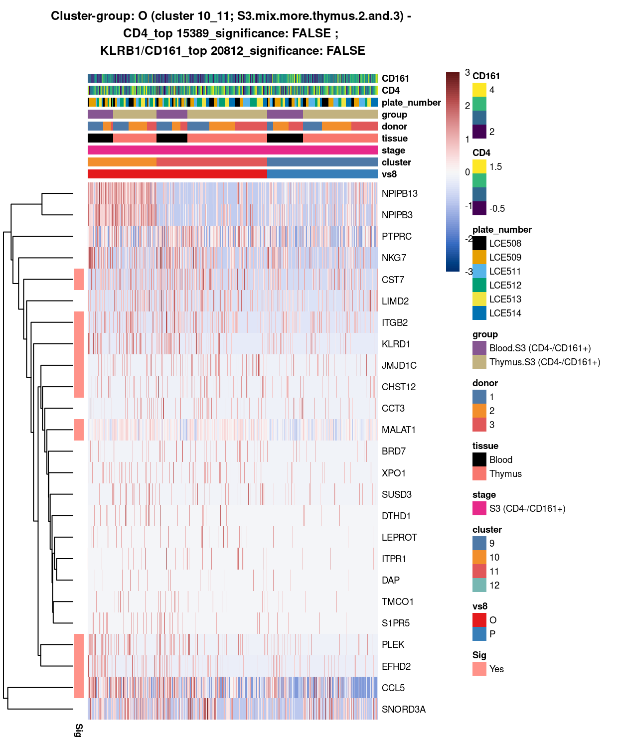
(#fig:heat-uniquely-up-logExp-cluster-10_11-vs-9)Heatmap of log-expression values in each sample for the top uniquely upregulated marker genes. Each column is a sample, each row a gene. Colours are capped at -3 and 3 to preserve dynamic range. Ranking of CD4 and CD161/KLRB1 from top of the DGE list sorted in ascending order of FDR and their statistical significance (TRUE = FDR < 0.05) are provided in the title.

Show code

##########################################################
# look at cluster-group P / cluster 9 (i.e. S3.mix.more.thymus.1)
chosen <- "P"
P_uniquely_up <- vs8_uniquely_up[[chosen]]

# add description for the chosen cluster-group
x <- "(cluster 9; S3.mix.more.thymus.1)"

# look only at protein coding gene (pcg)
# NOTE: not suggest to narrow down into pcg as it remove all significant candidates (FDR << 0.05) !
# P_uniquely_up_pcg <- P_uniquely_up[intersect(protein_coding_gene_set, rownames(P_uniquely_up)), ]

# get rid of noise (i.e. pseudo, ribo, mito, sex) that collaborator not interested in
P_uniquely_up_noiseR <- P_uniquely_up[setdiff(rownames(P_uniquely_up), c(pseudogene_set, mito_set, ribo_set, sex_set)), ]

# see if key marker, "CD4 and/or ""KLRB1/CD161"", contain in the DE list + if it is "significant (i.e FDR <0.05)
y <- c("CD4",
       which(rownames(P_uniquely_up_noiseR) %in% "CD4"),
       P_uniquely_up_noiseR[which(rownames(P_uniquely_up_noiseR) %in% "CD4"), ]$FDR < 0.05)
z <- c("KLRB1/CD161",
       which(rownames(P_uniquely_up_noiseR) %in% "KLRB1"),
       P_uniquely_up_noiseR[which(rownames(P_uniquely_up_noiseR) %in% "KLRB1"), ]$FDR < 0.05)

# top25 only + gene-of-interest
best_set <- P_uniquely_up_noiseR[1:25, ]

Show code

# heatmap
plotHeatmap(
  cp,
  features = rownames(best_set),
  columns = order(
    cp$vs8,
    cp$cluster,
    cp$stage,
    cp$tissue,
    cp$donor,
    cp$group,
    cp$plate_number,
    cp$CD4,
    cp$CD161),
  colour_columns_by = c(
    "vs8",
    "cluster",
    "stage",
    "tissue",
    "donor",
    "group",
    "plate_number",
    "CD4",
    "CD161"),
  cluster_cols = FALSE,
  center = TRUE,
  symmetric = TRUE,
  zlim = c(-3, 3),
  show_colnames = FALSE,
  annotation_row = data.frame(
    Sig = factor(
      ifelse(best_set[, "FDR"] < 0.05, "Yes", "No"),
      # TODO: temp trick to deal with the row-colouring problem
      # levels = c("Yes", "No")),
      levels = c("Yes")),
    row.names = rownames(best_set)),
  main = paste0("Cluster-group: ", chosen, " ", x, " - \n",
                y[1], "_top ", y[2], "_significance: ", y[3], " ; \n",
                z[1], "_top ", z[2], "_significance: ", z[3]),
  column_annotation_colors = list(
    # Sig = c("Yes" = "red", "No" = "lightgrey"),
    vs8 = vs8_colours,
    cluster = cluster_colours,
    stage = stage_colours,
    tissue = tissue_colours,
    donor = donor_colours,
    group = group_colours,
    plate_number = plate_number_colours),
  color = hcl.colors(101, "Blue-Red 3"),
  fontsize = 7)

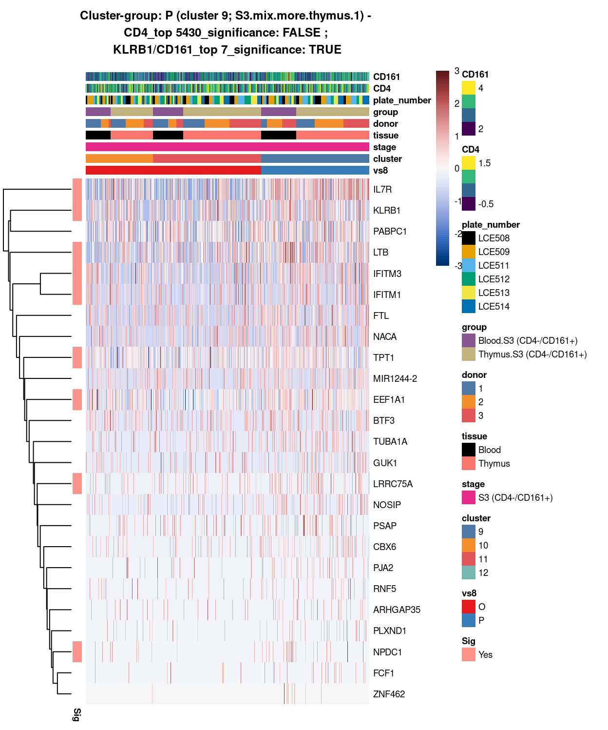
(#fig:heat-uniquely-up-logExp-cluster-9-vs-10_11)Heatmap of log-expression values in each sample for the top uniquely upregulated marker genes. Each column is a sample, each row a gene. Colours are capped at -3 and 3 to preserve dynamic range. Ranking of CD4 and CD161/KLRB1 from top of the DGE list sorted in ascending order of FDR and their statistical significance (TRUE = FDR < 0.05) are provided in the title.

DGE lists of these comparisons are available in output/marker_genes/S3_only/uniquely_up/cluster_10_11_vs_9/.

SUMMARY: 10_11 vs 9 (O vs P)

• cluster 10_11 (S3.mix.more.thymus.2.and.3 >>> got several marker significantly up-regulated in cluster 10_11 (e.g CCL5, EFHD2, CST7, ITGB2, etc.)
• cluster 9 (S3.mix.more.thymus.1 >>> got several markers as well (e.g. IL7R, LRRC75A; for LTB, IFITM3 and IFITM1, they seems to have higher expression in donor 3)
• COMMENT: cluster 9 clearly separated from 10_11, where 10 and 11 could be more similar; this can also explain why cluster 9 partner with 10 show no difference when compare to 11 !

cluster_9_11_vs_cluster_10

Show code

#########
# Q vs R
#########

##########################################################################################
# cluster 9_11 (i.e. S3.mix.more.thymus.1.and.3) vs cluster 10 (i.e. S3.mix.more.thymus.2)

# checkpoint
cp <- sce
# exclude cells of uninterested cluster from cp
cp <- cp[, cp$cluster == "9" | cp$cluster == "10" | cp$cluster == "11"]
colData(cp) <- droplevels(colData(cp))

# classify cluster-group for comparison
cp$vs9 <- factor(ifelse(cp$cluster == 9 | cp$cluster == 11, "Q", "R"))

# set vs colours
vs9_colours <- setNames(
  palette.colors(nlevels(cp$vs9), "Set1"),
  levels(cp$vs9))
cp$colours$vs9_colours <- vs9_colours[cp$vs9]

# find unique DE ./. cluster-groups
vs9_uniquely_up <- findMarkers(
  cp,
  groups = cp$vs9,
  block = cp$block,
  pval.type = "all",
  direction = "up")

# export DGE lists
saveRDS(
  vs9_uniquely_up,
  here("data", "marker_genes", "S3_only", "C094_Pellicci.uniquely_up.cluster_9_11_vs_10.rds"),
  compress = "xz")

dir.create(here("output", "marker_genes", "S3_only", "uniquely_up", "cluster_9_11_vs_10"), recursive = TRUE)

vs_pair <- c("9_11", "10")

message("Writing 'uniquely_up (cluster_9_11_vs_10)' marker genes to file.")
for (n in names(vs9_uniquely_up)) {
  message(n)
  gzout <- gzfile(
    description = here(
      "output",
      "marker_genes",
      "S3_only",
      "uniquely_up",
      "cluster_9_11_vs_10",
      paste0("cluster_",
             vs_pair[which(names(vs9_uniquely_up) %in% n)],
             "_vs_",
             vs_pair[-which(names(vs9_uniquely_up) %in% n)][1],
             ".uniquely_up.csv.gz")),
    open = "wb")
  write.table(
    x = vs9_uniquely_up[[n]] %>%
      as.data.frame() %>%
      tibble::rownames_to_column("gene_ID"),
    file = gzout,
    sep = ",",
    quote = FALSE,
    row.names = FALSE,
    col.names = TRUE)
  close(gzout)
}

Show code

###############################################################
# look at cluster-group Q / cluster 9_11 (i.e. S3.mix.more.thymus.1.and.3)
chosen <- "Q"
Q_uniquely_up <- vs9_uniquely_up[[chosen]]

# add description for the chosen cluster-group
x <- "(cluster 9_11; S3.mix.more.thymus.1.and.3)"

# look only at protein coding gene (pcg)
# NOTE: not suggest to narrow down into pcg as it remove all significant candidates (FDR << 0.05) !
# Q_uniquely_up_pcg <- Q_uniquely_up[intersect(protein_coding_gene_set, rownames(Q_uniquely_up)), ]

# get rid of noise (i.e. pseudo, ribo, mito, sex) that collaborator not interested in
Q_uniquely_up_noiseR <- Q_uniquely_up[setdiff(rownames(Q_uniquely_up), c(pseudogene_set, mito_set, ribo_set, sex_set)), ]

# see if key marker, "CD4 and/or ""KLRB1/CD161"", contain in the DE list + if it is "significant (i.e FDR <0.05)
y <- c("CD4",
       which(rownames(Q_uniquely_up_noiseR) %in% "CD4"),
       Q_uniquely_up_noiseR[which(rownames(Q_uniquely_up_noiseR) %in% "CD4"), ]$FDR < 0.05)
z <- c("KLRB1/CD161",
       which(rownames(Q_uniquely_up_noiseR) %in% "KLRB1"),
       Q_uniquely_up_noiseR[which(rownames(Q_uniquely_up_noiseR) %in% "KLRB1"), ]$FDR < 0.05)

# top25 only + gene-of-interest
best_set <- Q_uniquely_up_noiseR[1:25, ]

Show code

# heatmap
plotHeatmap(
  cp,
  features = rownames(best_set),
  columns = order(
    cp$vs9,
    cp$cluster,
    cp$stage,
    cp$tissue,
    cp$donor,
    cp$group,
    cp$plate_number,
    cp$CD4,
    cp$CD161),
  colour_columns_by = c(
    "vs9",
    "cluster",
    "stage",
    "tissue",
    "donor",
    "group",
    "plate_number",
    "CD4",
    "CD161"),
  cluster_cols = FALSE,
  center = TRUE,
  symmetric = TRUE,
  zlim = c(-3, 3),
  show_colnames = FALSE,
  annotation_row = data.frame(
    Sig = factor(
      ifelse(best_set[, "FDR"] < 0.05, "Yes", "No"),
      # TODO: temp trick to deal with the row-colouring problem
      # levels = c("Yes", "No")),
      levels = c("Yes")),
    row.names = rownames(best_set)),
  main = paste0("Cluster-group: ", chosen, " ", x, " - \n",
                y[1], "_top ", y[2], "_significance: ", y[3], " ; \n",
                z[1], "_top ", z[2], "_significance: ", z[3]),
  column_annotation_colors = list(
    # Sig = c("Yes" = "red", "No" = "lightgrey"),
    vs9 = vs9_colours,
    cluster = cluster_colours,
    stage = stage_colours,
    tissue = tissue_colours,
    donor = donor_colours,
    group = group_colours,
    plate_number = plate_number_colours),
  color = hcl.colors(101, "Blue-Red 3"),
  fontsize = 7)

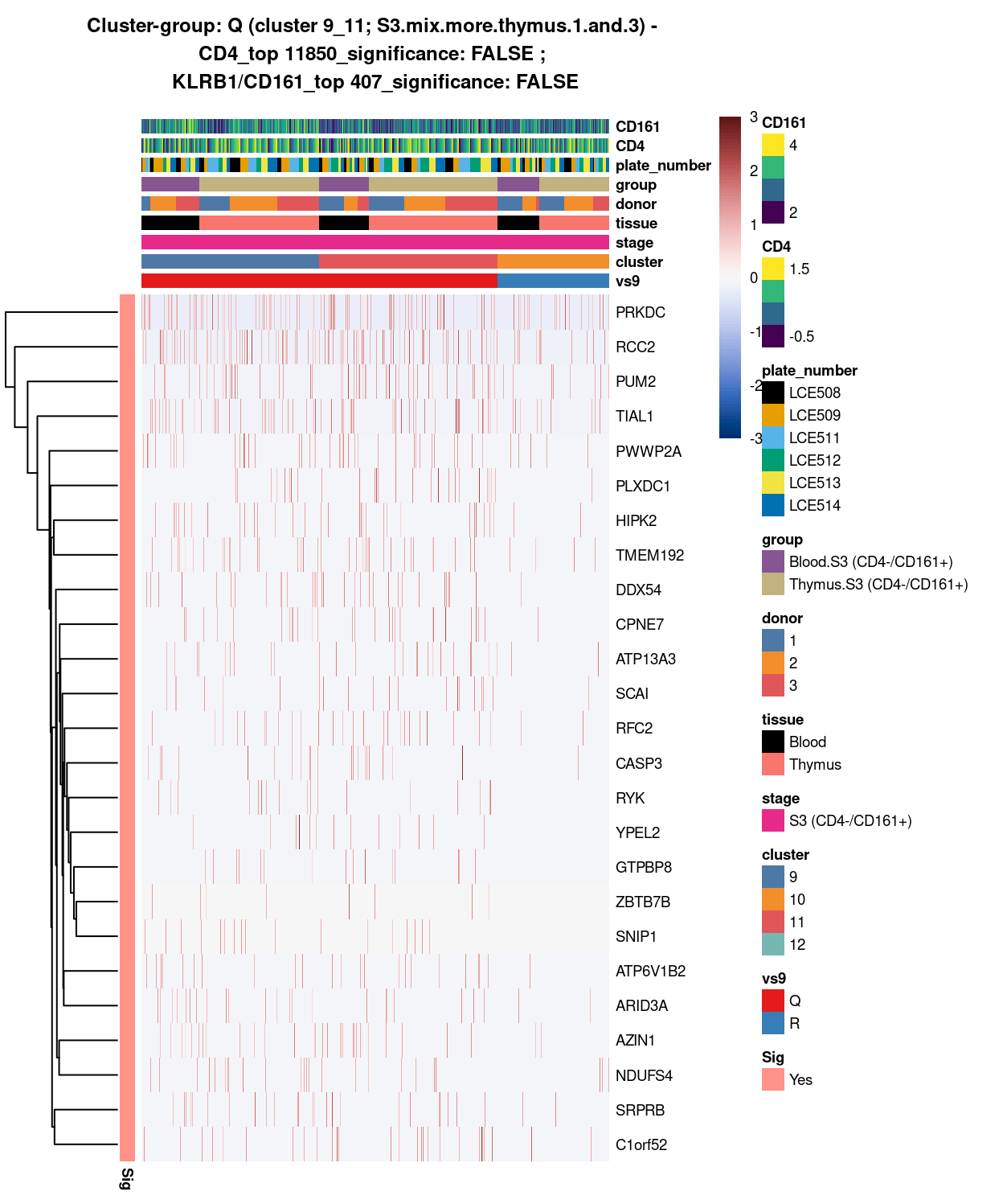
(#fig:heat-uniquely-up-logExp-cluster-9_11-vs-10)Heatmap of log-expression values in each sample for the top uniquely upregulated marker genes. Each column is a sample, each row a gene. Colours are capped at -3 and 3 to preserve dynamic range. Ranking of CD4 and CD161/KLRB1 from top of the DGE list sorted in ascending order of FDR and their statistical significance (TRUE = FDR < 0.05) are provided in the title.

Show code

##########################################################
# look at cluster-group R / cluster 10 (i.e. S3.mix.more.thymus.2)
chosen <- "R"
R_uniquely_up <- vs9_uniquely_up[[chosen]]

# add description for the chosen cluster-group
x <- "(cluster 10; S3.mix.more.thymus.2)"

# look only at protein coding gene (pcg)
# NOTE: not suggest to narrow down into pcg as it remove all significant candidates (FDR << 0.05) !
# R_uniquely_up_pcg <- R_uniquely_up[intersect(protein_coding_gene_set, rownames(R_uniquely_up)), ]

# get rid of noise (i.e. pseudo, ribo, mito, sex) that collaborator not interested in
R_uniquely_up_noiseR <- R_uniquely_up[setdiff(rownames(R_uniquely_up), c(pseudogene_set, mito_set, ribo_set, sex_set)), ]

# see if key marker, "CD4 and/or ""KLRB1/CD161"", contain in the DE list + if it is "significant (i.e FDR <0.05)
y <- c("CD4",
       which(rownames(R_uniquely_up_noiseR) %in% "CD4"),
       R_uniquely_up_noiseR[which(rownames(R_uniquely_up_noiseR) %in% "CD4"), ]$FDR < 0.05)
z <- c("KLRB1/CD161",
       which(rownames(R_uniquely_up_noiseR) %in% "KLRB1"),
       R_uniquely_up_noiseR[which(rownames(R_uniquely_up_noiseR) %in% "KLRB1"), ]$FDR < 0.05)

# top25 only + gene-of-interest
best_set <- R_uniquely_up_noiseR[1:25, ]

Show code

# heatmap
plotHeatmap(
  cp,
  features = rownames(best_set),
  columns = order(
    cp$vs9,
    cp$cluster,
    cp$stage,
    cp$tissue,
    cp$donor,
    cp$group,
    cp$plate_number,
    cp$CD4,
    cp$CD161),
  colour_columns_by = c(
    "vs9",
    "cluster",
    "stage",
    "tissue",
    "donor",
    "group",
    "plate_number",
    "CD4",
    "CD161"),
  cluster_cols = FALSE,
  center = TRUE,
  symmetric = TRUE,
  zlim = c(-3, 3),
  show_colnames = FALSE,
  annotation_row = data.frame(
    Sig = factor(
      ifelse(best_set[, "FDR"] < 0.05, "Yes", "No"),
      # TODO: temp trick to deal with the row-colouring problem
      # levels = c("Yes", "No")),
      levels = c("Yes")),
    row.names = rownames(best_set)),
  main = paste0("Cluster-group: ", chosen, " ", x, " - \n",
                y[1], "_top ", y[2], "_significance: ", y[3], " ; \n",
                z[1], "_top ", z[2], "_significance: ", z[3]),
  column_annotation_colors = list(
    # Sig = c("Yes" = "red", "No" = "lightgrey"),
    vs9 = vs9_colours,
    cluster = cluster_colours,
    stage = stage_colours,
    tissue = tissue_colours,
    donor = donor_colours,
    group = group_colours,
    plate_number = plate_number_colours),
  color = hcl.colors(101, "Blue-Red 3"),
  fontsize = 7)

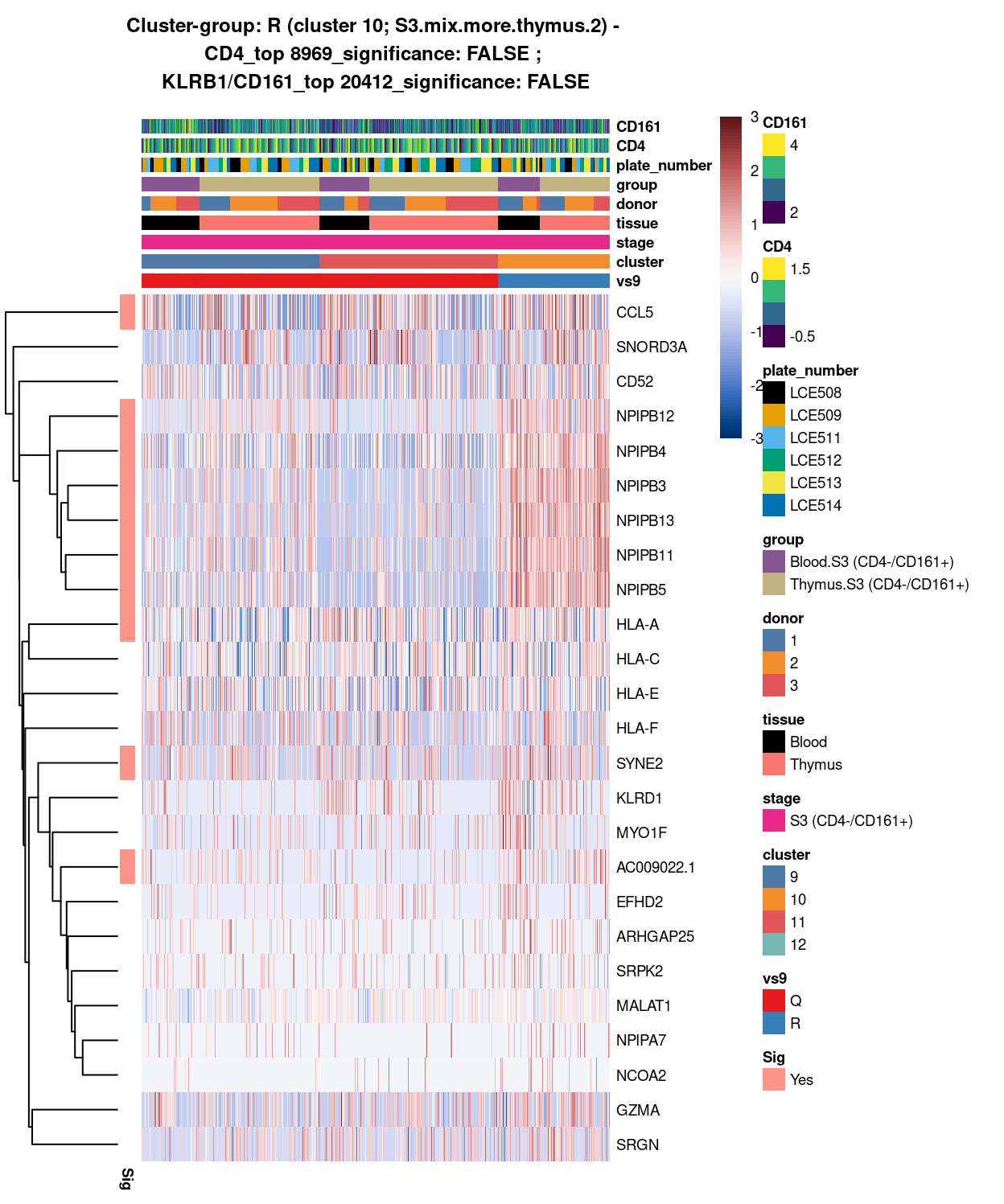
(#fig:heat-uniquely-up-logExp-cluster-10-vs-9_11)Heatmap of log-expression values in each sample for the top uniquely upregulated marker genes. Each column is a sample, each row a gene. Colours are capped at -3 and 3 to preserve dynamic range. Ranking of CD4 and CD161/KLRB1 from top of the DGE list sorted in ascending order of FDR and their statistical significance (TRUE = FDR < 0.05) are provided in the title.

DGE lists of these comparisons are available in output/marker_genes/S3_only/uniquely_up/cluster_9_11_vs_10/.

SUMMARY: 9_11 vs 10 (Q vs R)

• cluster 9_11 (S3.mix.more.thymus.1.and.3 >>> lots of markers significantly up-regulated in cluster 9_11 (e.g. PRKDC, SCAI, DDX54)
• cluster 10 (S3.mix.more.thymus.2 >>> besides NPIPB family member, it got CCL5, SYNE2 and AC009022.9 as its markers
• COMMENT: if cluster 11 is in the combination, it returns DE; does this means … cluster 11 is more different from cluster 9 or 10 ?

cluster_9_10_vs_cluster_12

Show code

#########
# S vs T
#########

##########################################################################################
# cluster 9_10 (i.e. S3.mix.more.thymus.1) vs cluster 12 (i.e. S3.mix.more.thymus.4.center)

# checkpoint
cp <- sce
# exclude cells of uninterested cluster from cp
cp <- cp[, cp$cluster == "9" | cp$cluster == "10" | cp$cluster == "12"]
colData(cp) <- droplevels(colData(cp))

# classify cluster-group for comparison
cp$vs10 <- factor(ifelse(cp$cluster == 9 | cp$cluster == 10, "S", "T"))

# set vs colours
vs10_colours <- setNames(
  palette.colors(nlevels(cp$vs10), "Set1"),
  levels(cp$vs10))
cp$colours$vs10_colours <- vs10_colours[cp$vs10]

# find unique DE ./. cluster-groups
vs10_uniquely_up <- findMarkers(
  cp,
  groups = cp$vs10,
  block = cp$block,
  pval.type = "all",
  direction = "up")

# export DGE lists
saveRDS(
  vs10_uniquely_up,
  here("data", "marker_genes", "S3_only", "C094_Pellicci.uniquely_up.cluster_9_10_vs_12.rds"),
  compress = "xz")

dir.create(here("output", "marker_genes", "S3_only", "uniquely_up", "cluster_9_10_vs_12"), recursive = TRUE)

vs_pair <- c("9_10", "12")

message("Writing 'uniquely_up (cluster_9_10_vs_12)' marker genes to file.")
for (n in names(vs10_uniquely_up)) {
  message(n)
  gzout <- gzfile(
    description = here(
      "output",
      "marker_genes",
      "S3_only",
      "uniquely_up",
      "cluster_9_10_vs_12",
      paste0("cluster_",
             vs_pair[which(names(vs10_uniquely_up) %in% n)],
             "_vs_",
             vs_pair[-which(names(vs10_uniquely_up) %in% n)][1],
             ".uniquely_up.csv.gz")),
    open = "wb")
  write.table(
    x = vs10_uniquely_up[[n]] %>%
      as.data.frame() %>%
      tibble::rownames_to_column("gene_ID"),
    file = gzout,
    sep = ",",
    quote = FALSE,
    row.names = FALSE,
    col.names = TRUE)
  close(gzout)
}

Show code

###############################################################
# look at cluster-group S / cluster 9_10 (i.e. S3.mix.more.thymus.1.and.2)
chosen <- "S"
S_uniquely_up <- vs10_uniquely_up[[chosen]]

# add description for the chosen cluster-group
x <- "(cluster 9_10; S3.mix.more.thymus.1.and.2)"

# look only at protein coding gene (pcg)
# NOTE: not suggest to narrow down into pcg as it remove all significant candidates (FDR << 0.05) !
# S_uniquely_up_pcg <- S_uniquely_up[intersect(protein_coding_gene_set, rownames(S_uniquely_up)), ]

# get rid of noise (i.e. pseudo, ribo, mito, sex) that collaborator not interested in
S_uniquely_up_noiseR <- S_uniquely_up[setdiff(rownames(S_uniquely_up), c(pseudogene_set, mito_set, ribo_set, sex_set)), ]

# see if key marker, "CD4 and/or ""KLRB1/CD161"", contain in the DE list + if it is "significant (i.e FDR <0.05)
y <- c("CD4",
       which(rownames(S_uniquely_up_noiseR) %in% "CD4"),
       S_uniquely_up_noiseR[which(rownames(S_uniquely_up_noiseR) %in% "CD4"), ]$FDR < 0.05)
z <- c("KLRB1/CD161",
       which(rownames(S_uniquely_up_noiseR) %in% "KLRB1"),
       S_uniquely_up_noiseR[which(rownames(S_uniquely_up_noiseR) %in% "KLRB1"), ]$FDR < 0.05)

# top25 only + gene-of-interest
best_set <- S_uniquely_up_noiseR[1:25, ]

Show code

# heatmap
plotHeatmap(
  cp,
  features = rownames(best_set),
  columns = order(
    cp$vs10,
    cp$cluster,
    cp$stage,
    cp$tissue,
    cp$donor,
    cp$group,
    cp$plate_number,
    cp$CD4,
    cp$CD161),
  colour_columns_by = c(
    "vs10",
    "cluster",
    "stage",
    "tissue",
    "donor",
    "group",
    "plate_number",
    "CD4",
    "CD161"),
  cluster_cols = FALSE,
  center = TRUE,
  symmetric = TRUE,
  zlim = c(-3, 3),
  show_colnames = FALSE,
  annotation_row = data.frame(
    Sig = factor(
      ifelse(best_set[, "FDR"] < 0.05, "Yes", "No"),
      # TODO: temp trick to deal with the row-colouring problem
      # levels = c("Yes", "No")),
      levels = c("Yes")),
    row.names = rownames(best_set)),
  main = paste0("Cluster-group: ", chosen, " ", x, " - \n",
                y[1], "_top ", y[2], "_significance: ", y[3], " ; \n",
                z[1], "_top ", z[2], "_significance: ", z[3]),
  column_annotation_colors = list(
    # Sig = c("Yes" = "red", "No" = "lightgrey"),
    vs10 = vs10_colours,
    cluster = cluster_colours,
    stage = stage_colours,
    tissue = tissue_colours,
    donor = donor_colours,
    group = group_colours,
    plate_number = plate_number_colours),
  color = hcl.colors(101, "Blue-Red 3"),
  fontsize = 7)

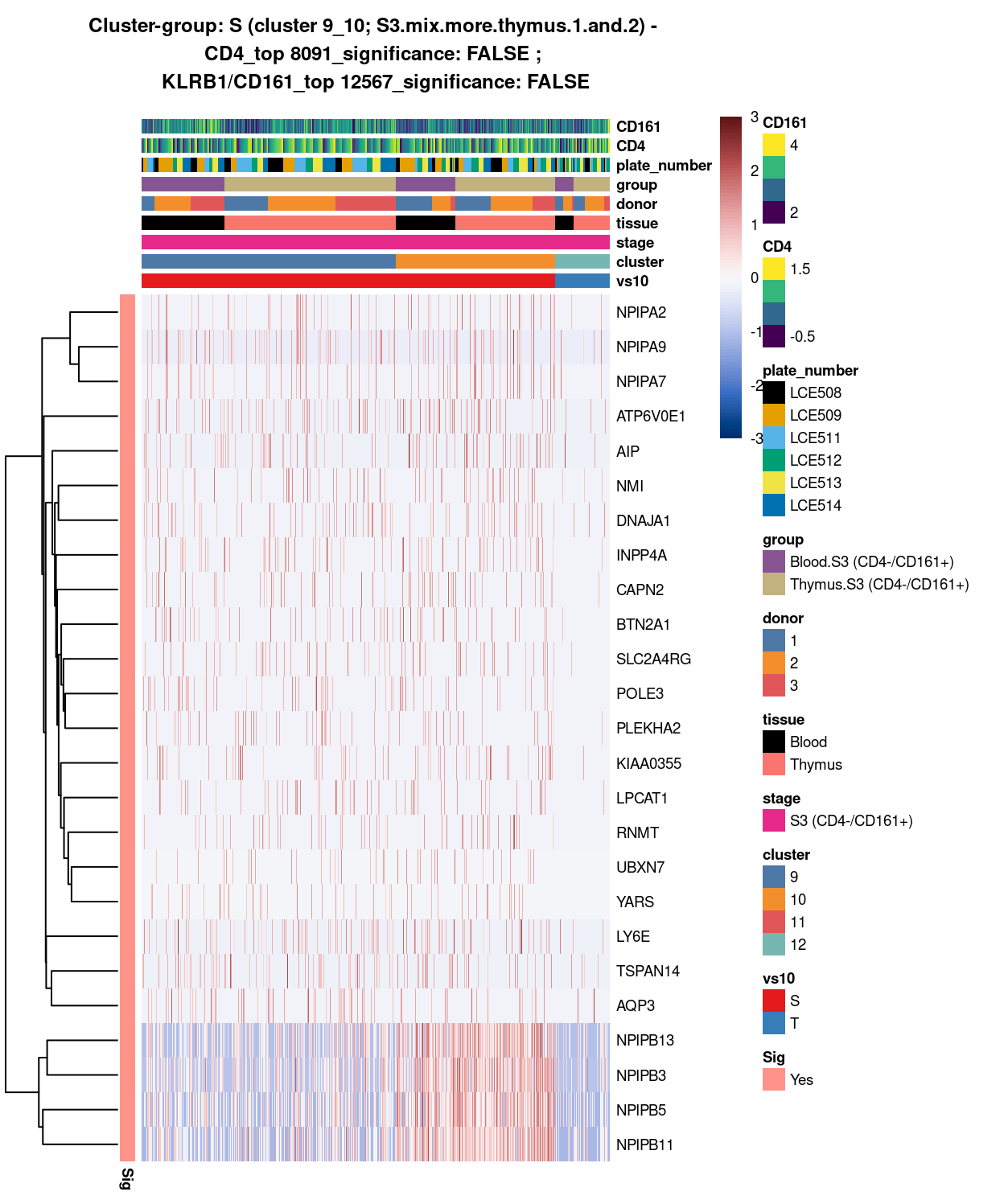
(#fig:heat-uniquely-up-logExp-cluster-9_10-vs-12)Heatmap of log-expression values in each sample for the top uniquely upregulated marker genes. Each column is a sample, each row a gene. Colours are capped at -3 and 3 to preserve dynamic range. Ranking of CD4 and CD161/KLRB1 from top of the DGE list sorted in ascending order of FDR and their statistical significance (TRUE = FDR < 0.05) are provided in the title.

Show code

##########################################################
# look at cluster-group T / cluster 12 (i.e. S3.mix.more.thymus.4.center)
chosen <- "T"
T_uniquely_up <- vs10_uniquely_up[[chosen]]

# add description for the chosen cluster-group
x <- "(cluster 12; S3.mix.more.thymus.4.center)"

# look only at protein coding gene (pcg)
# NOTE: not suggest to narrow down into pcg as it remove all significant candidates (FDR << 0.05) !
# T_uniquely_up_pcg <- T_uniquely_up[intersect(protein_coding_gene_set, rownames(T_uniquely_up)), ]

# get rid of noise (i.e. pseudo, ribo, mito, sex) that collaborator not interested in
T_uniquely_up_noiseR <- T_uniquely_up[setdiff(rownames(T_uniquely_up), c(pseudogene_set, mito_set, ribo_set, sex_set)), ]

# see if key marker, "CD4 and/or ""KLRB1/CD161"", contain in the DE list + if it is "significant (i.e FDR <0.05)
y <- c("CD4",
       which(rownames(T_uniquely_up_noiseR) %in% "CD4"),
       T_uniquely_up_noiseR[which(rownames(T_uniquely_up_noiseR) %in% "CD4"), ]$FDR < 0.05)
z <- c("KLRB1/CD161",
       which(rownames(T_uniquely_up_noiseR) %in% "KLRB1"),
       T_uniquely_up_noiseR[which(rownames(T_uniquely_up_noiseR) %in% "KLRB1"), ]$FDR < 0.05)

# top25 only + gene-of-interest
best_set <- T_uniquely_up_noiseR[1:25, ]

Show code

# heatmap
plotHeatmap(
  cp,
  features = rownames(best_set),
  columns = order(
    cp$vs10,
    cp$cluster,
    cp$stage,
    cp$tissue,
    cp$donor,
    cp$group,
    cp$plate_number,
    cp$CD4,
    cp$CD161),
  colour_columns_by = c(
    "vs10",
    "cluster",
    "stage",
    "tissue",
    "donor",
    "group",
    "plate_number",
    "CD4",
    "CD161"),
  cluster_cols = FALSE,
  center = TRUE,
  symmetric = TRUE,
  zlim = c(-3, 3),
  show_colnames = FALSE,
  annotation_row = data.frame(
    Sig = factor(
      ifelse(best_set[, "FDR"] < 0.05, "Yes", "No"),
      # TODO: temp trick to deal with the row-colouring problem
      # levels = c("Yes", "No")),
      levels = c("Yes")),
    row.names = rownames(best_set)),
  main = paste0("Cluster-group: ", chosen, " ", x, " - \n",
                y[1], "_top ", y[2], "_significance: ", y[3], " ; \n",
                z[1], "_top ", z[2], "_significance: ", z[3]),
  column_annotation_colors = list(
    # Sig = c("Yes" = "red", "No" = "lightgrey"),
    vs10 = vs10_colours,
    cluster = cluster_colours,
    stage = stage_colours,
    tissue = tissue_colours,
    donor = donor_colours,
    group = group_colours,
    plate_number = plate_number_colours),
  color = hcl.colors(101, "Blue-Red 3"),
  fontsize = 7)

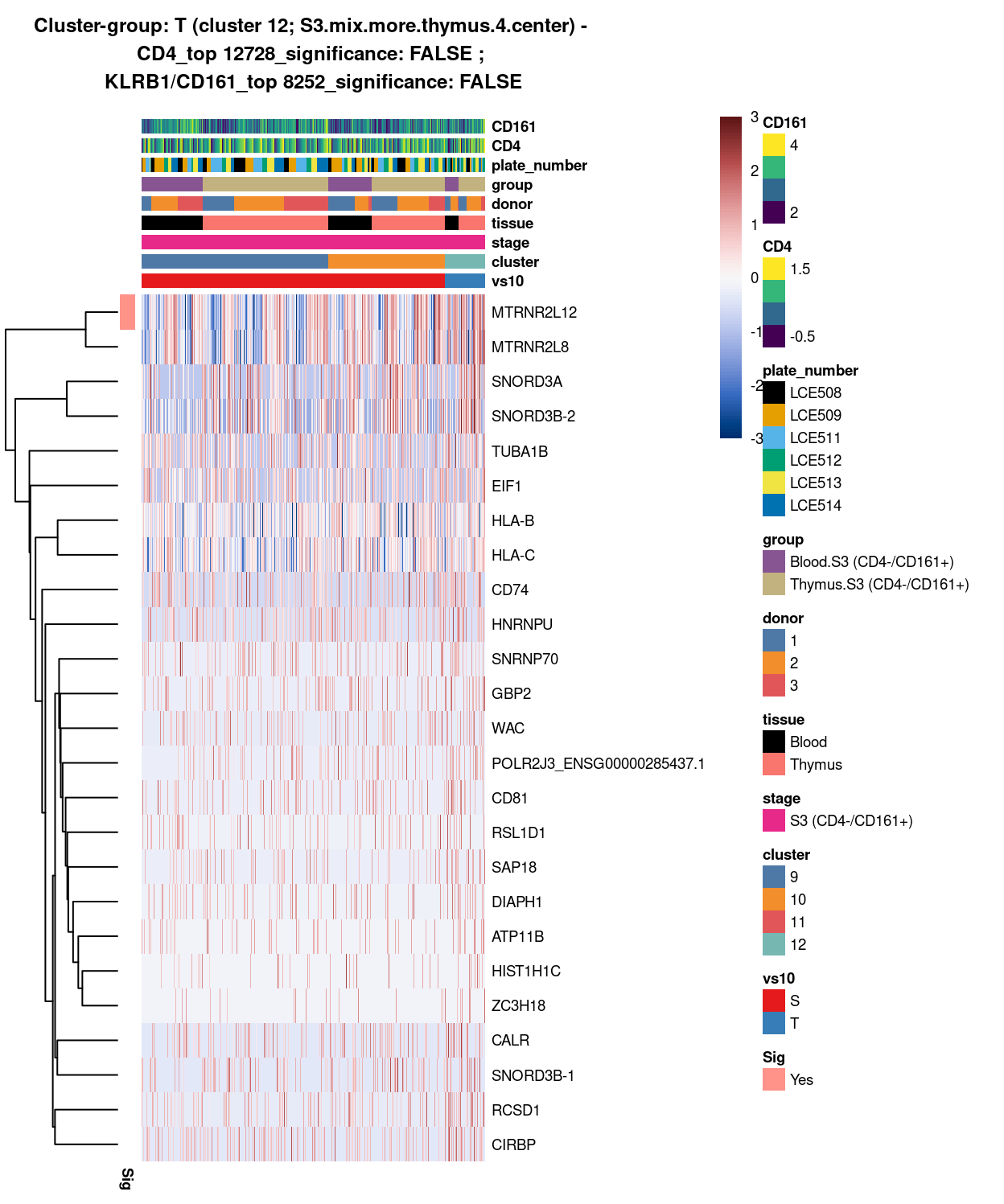
(#fig:heat-uniquely-up-logExp-cluster-12-vs-9_10)Heatmap of log-expression values in each sample for the top uniquely upregulated marker genes. Each column is a sample, each row a gene. Colours are capped at -3 and 3 to preserve dynamic range. Ranking of CD4 and CD161/KLRB1 from top of the DGE list sorted in ascending order of FDR and their statistical significance (TRUE = FDR < 0.05) are provided in the title.

DGE lists of these comparisons are available in output/marker_genes/S3_only/uniquely_up/cluster_9_10_vs_12/.

SUMMARY: 9_10 vs 12 (S vs T)

• cluster 9_10 (S3.mix.more.thymus.1.and.2 >>> lot of markers on cluster 9_10 (e/g/ AIP, NIM, POLE3, etc.)
• cluster 12 (S3.mix.more.thymus.4 >>> except for the mitochondrial gene, no statistically significant markers found
• COMMENT: consistently, 12 show no marker, uniqueness is from cluster 9_10

cluster_10_11_vs_cluster_12

Show code

#########
# U vs V
#########

##########################################################################################
# cluster 10_11 (i.e. S3.mix.more.thymus.2.and.3) vs cluster 12 (i.e. S3.mix.more.thymus.4.center)

# checkpoint
cp <- sce
# exclude cells of uninterested cluster from cp
cp <- cp[, cp$cluster == "10" | cp$cluster == "11" | cp$cluster == "12"]
colData(cp) <- droplevels(colData(cp))

# classify cluster-group for comparison
cp$vs11 <- factor(ifelse(cp$cluster == 10 | cp$cluster == 11, "U", "V"))

# set vs colours
vs11_colours <- setNames(
  palette.colors(nlevels(cp$vs11), "Set1"),
  levels(cp$vs11))
cp$colours$vs11_colours <- vs11_colours[cp$vs11]

# find unique DE ./. cluster-groups
vs11_uniquely_up <- findMarkers(
  cp,
  groups = cp$vs11,
  block = cp$block,
  pval.type = "all",
  direction = "up")

# export DGE lists
saveRDS(
  vs11_uniquely_up,
  here("data", "marker_genes", "S3_only", "C094_Pellicci.uniquely_up.cluster_10_11_vs_12.rds"),
  compress = "xz")

dir.create(here("output", "marker_genes", "S3_only", "uniquely_up", "cluster_10_11_vs_12"), recursive = TRUE)

vs_pair <- c("10_11", "12")

message("Writing 'uniquely_up (cluster_10_11_vs_12)' marker genes to file.")
for (n in names(vs11_uniquely_up)) {
  message(n)
  gzout <- gzfile(
    description = here(
      "output",
      "marker_genes",
      "S3_only",
      "uniquely_up",
      "cluster_10_11_vs_12",
      paste0("cluster_",
             vs_pair[which(names(vs11_uniquely_up) %in% n)],
             "_vs_",
             vs_pair[-which(names(vs11_uniquely_up) %in% n)][1],
             ".uniquely_up.csv.gz")),
    open = "wb")
  write.table(
    x = vs11_uniquely_up[[n]] %>%
      as.data.frame() %>%
      tibble::rownames_to_column("gene_ID"),
    file = gzout,
    sep = ",",
    quote = FALSE,
    row.names = FALSE,
    col.names = TRUE)
  close(gzout)
}

Show code

###############################################################
# look at cluster-group U / cluster 10_11 (i.e. S3.mix.more.thymus.2.and.3)
chosen <- "U"
U_uniquely_up <- vs11_uniquely_up[[chosen]]

# add description for the chosen cluster-group
x <- "(cluster 10_11; S3.mix.more.thymus.2.and.3)"

# look only at protein coding gene (pcg)
# NOTE: not suggest to narrow down into pcg as it remove all significant candidates (FDR << 0.05) !
# U_uniquely_up_pcg <- U_uniquely_up[intersect(protein_coding_gene_set, rownames(U_uniquely_up)), ]

# get rid of noise (i.e. pseudo, ribo, mito, sex) that collaborator not interested in
U_uniquely_up_noiseR <- U_uniquely_up[setdiff(rownames(U_uniquely_up), c(pseudogene_set, mito_set, ribo_set, sex_set)), ]

# see if key marker, "CD4 and/or ""KLRB1/CD161"", contain in the DE list + if it is "significant (i.e FDR <0.05)
y <- c("CD4",
       which(rownames(U_uniquely_up_noiseR) %in% "CD4"),
       U_uniquely_up_noiseR[which(rownames(U_uniquely_up_noiseR) %in% "CD4"), ]$FDR < 0.05)
z <- c("KLRB1/CD161",
       which(rownames(U_uniquely_up_noiseR) %in% "KLRB1"),
       U_uniquely_up_noiseR[which(rownames(U_uniquely_up_noiseR) %in% "KLRB1"), ]$FDR < 0.05)

# top25 only + gene-of-interest
best_set <- U_uniquely_up_noiseR[1:25, ]

Show code

# heatmap
plotHeatmap(
  cp,
  features = rownames(best_set),
  columns = order(
    cp$vs11,
    cp$cluster,
    cp$stage,
    cp$tissue,
    cp$donor,
    cp$group,
    cp$plate_number,
    cp$CD4,
    cp$CD161),
  colour_columns_by = c(
    "vs11",
    "cluster",
    "stage",
    "tissue",
    "donor",
    "group",
    "plate_number",
    "CD4",
    "CD161"),
  cluster_cols = FALSE,
  center = TRUE,
  symmetric = TRUE,
  zlim = c(-3, 3),
  show_colnames = FALSE,
  annotation_row = data.frame(
    Sig = factor(
      ifelse(best_set[, "FDR"] < 0.05, "Yes", "No"),
      # TODO: temp trick to deal with the row-colouring problem
      # levels = c("Yes", "No")),
      levels = c("Yes")),
    row.names = rownames(best_set)),
  main = paste0("Cluster-group: ", chosen, " ", x, " - \n",
                y[1], "_top ", y[2], "_significance: ", y[3], " ; \n",
                z[1], "_top ", z[2], "_significance: ", z[3]),
  column_annotation_colors = list(
    # Sig = c("Yes" = "red", "No" = "lightgrey"),
    vs11 = vs11_colours,
    cluster = cluster_colours,
    stage = stage_colours,
    tissue = tissue_colours,
    donor = donor_colours,
    group = group_colours,
    plate_number = plate_number_colours),
  color = hcl.colors(101, "Blue-Red 3"),
  fontsize = 7)

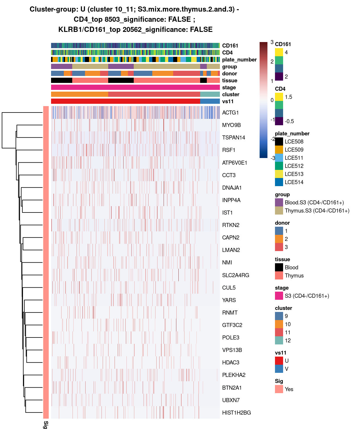
(#fig:heat-uniquely-up-logExp-cluster-10_11-vs-12)Heatmap of log-expression values in each sample for the top uniquely upregulated marker genes. Each column is a sample, each row a gene. Colours are capped at -3 and 3 to preserve dynamic range. Ranking of CD4 and CD161/KLRB1 from top of the DGE list sorted in ascending order of FDR and their statistical significance (TRUE = FDR < 0.05) are provided in the title.

Show code

##########################################################
# look at cluster-group V / cluster 12 (i.e. S3.mix.more.thymus.4.center)
chosen <- "V"
V_uniquely_up <- vs11_uniquely_up[[chosen]]

# add description for the chosen cluster-group
x <- "(cluster 12; S3.mix.more.thymus.4.center)"

# look only at protein coding gene (pcg)
# NOTE: not suggest to narrow down into pcg as it remove all significant candidates (FDR << 0.05) !
# V_uniquely_up_pcg <- V_uniquely_up[intersect(protein_coding_gene_set, rownames(V_uniquely_up)), ]

# get rid of noise (i.e. pseudo, ribo, mito, sex) that collaborator not interested in
V_uniquely_up_noiseR <- V_uniquely_up[setdiff(rownames(V_uniquely_up), c(pseudogene_set, mito_set, ribo_set, sex_set)), ]

# see if key marker, "CD4 and/or ""KLRB1/CD161"", contain in the DE list + if it is "significant (i.e FDR <0.05)
y <- c("CD4",
       which(rownames(V_uniquely_up_noiseR) %in% "CD4"),
       V_uniquely_up_noiseR[which(rownames(V_uniquely_up_noiseR) %in% "CD4"), ]$FDR < 0.05)
z <- c("KLRB1/CD161",
       which(rownames(V_uniquely_up_noiseR) %in% "KLRB1"),
       V_uniquely_up_noiseR[which(rownames(V_uniquely_up_noiseR) %in% "KLRB1"), ]$FDR < 0.05)

# top25 only + gene-of-interest
best_set <- V_uniquely_up_noiseR[1:25, ]

Show code

# heatmap
plotHeatmap(
  cp,
  features = rownames(best_set),
  columns = order(
    cp$vs11,
    cp$cluster,
    cp$stage,
    cp$tissue,
    cp$donor,
    cp$group,
    cp$plate_number,
    cp$CD4,
    cp$CD161),
  colour_columns_by = c(
    "vs11",
    "cluster",
    "stage",
    "tissue",
    "donor",
    "group",
    "plate_number",
    "CD4",
    "CD161"),
  cluster_cols = FALSE,
  center = TRUE,
  symmetric = TRUE,
  zlim = c(-3, 3),
  show_colnames = FALSE,
  # annotation_row = data.frame(
  #   Sig = factor(
  #     ifelse(best_set[, "FDR"] < 0.05, "Yes", "No"),
  #     # TODO: temp trick to deal with the row-colouring problem
  #     # levels = c("Yes", "No")),
  #     levels = c("Yes")),
  #   row.names = rownames(best_set)),
  main = paste0("Cluster-group: ", chosen, " ", x, " - \n",
                y[1], "_top ", y[2], "_significance: ", y[3], " ; \n",
                z[1], "_top ", z[2], "_significance: ", z[3]),
  column_annotation_colors = list(
    # Sig = c("Yes" = "red", "No" = "lightgrey"),
    vs11 = vs11_colours,
    cluster = cluster_colours,
    stage = stage_colours,
    tissue = tissue_colours,
    donor = donor_colours,
    group = group_colours,
    plate_number = plate_number_colours),
  color = hcl.colors(101, "Blue-Red 3"),
  fontsize = 7)

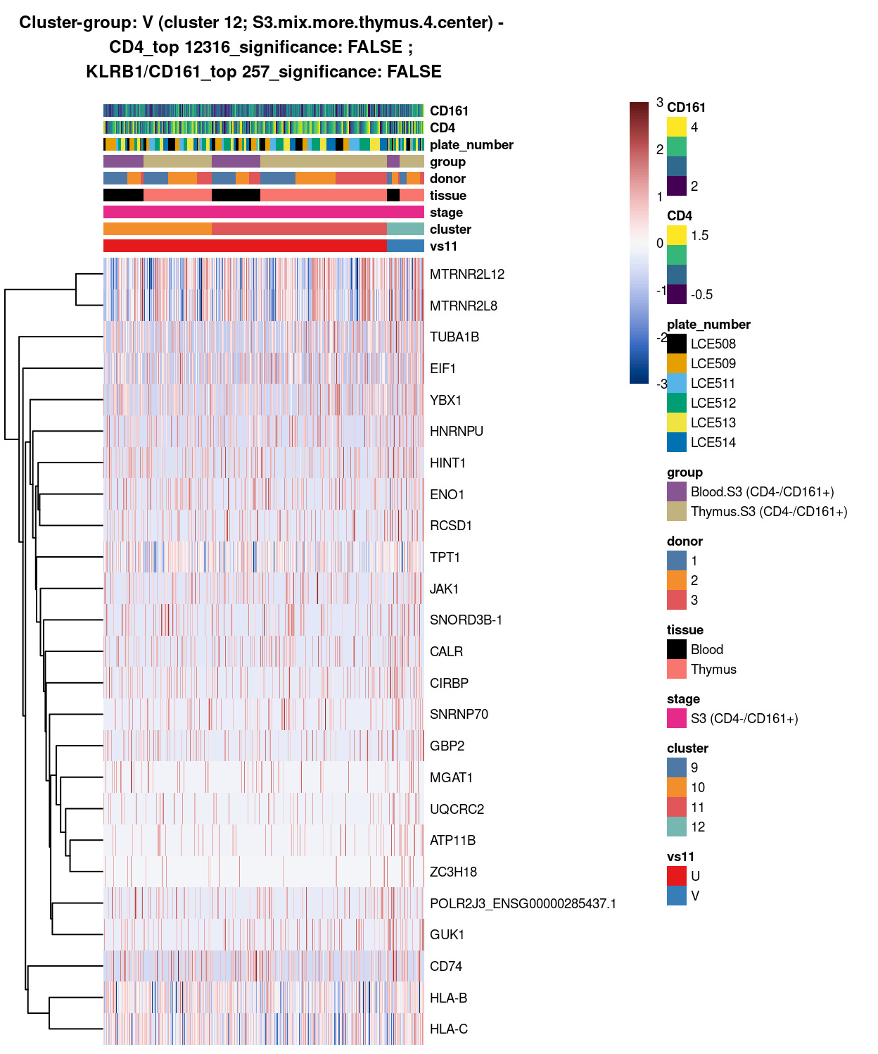
(#fig:heat-uniquely-up-logExp-cluster-12-vs-10_11)Heatmap of log-expression values in each sample for the top uniquely upregulated marker genes. Each column is a sample, each row a gene. Colours are capped at -3 and 3 to preserve dynamic range. Ranking of CD4 and CD161/KLRB1 from top of the DGE list sorted in ascending order of FDR and their statistical significance (TRUE = FDR < 0.05) are provided in the title.

DGE lists of these comparisons are available in output/marker_genes/S3_only/uniquely_up/cluster_10_11_vs_12/.

SUMMARY: 10_11 vs 12 (U vs V)

• cluster 10_11 (S3.mix.more.thymus.2.and.3 >>> lots of markers significantly up-regulated in 10_11
• cluster 12 (S3.mix.more.thymus.4 >>> no statistically significant marker found on this centered cluster
• COMMENT: consistently, cluster 12 show no marker, uniqueness is from cluster 10_11

cluster_9_11_vs_cluster_12

Show code

#########
# W vs X
#########

##########################################################################################
# cluster 9_11 (i.e. S3.mix.more.thymus.1.and.3) vs cluster 12 (i.e. S3.mix.more.thymus.4.center)

# checkpoint
cp <- sce
# exclude cells of uninterested cluster from cp
cp <- cp[, cp$cluster == "9" | cp$cluster == "11" | cp$cluster == "12"]
colData(cp) <- droplevels(colData(cp))

# classify cluster-group for comparison
cp$vs12 <- factor(ifelse(cp$cluster == 9 | cp$cluster == 11, "W", "X"))

# set vs colours
vs12_colours <- setNames(
  palette.colors(nlevels(cp$vs12), "Set1"),
  levels(cp$vs12))
cp$colours$vs12_colours <- vs12_colours[cp$vs12]

# find unique DE ./. cluster-groups
vs12_uniquely_up <- findMarkers(
  cp,
  groups = cp$vs12,
  block = cp$block,
  pval.type = "all",
  direction = "up")

# export DGE lists
saveRDS(
  vs12_uniquely_up,
  here("data", "marker_genes", "S3_only", "C094_Pellicci.uniquely_up.cluster_9_11_vs_12.rds"),
  compress = "xz")

dir.create(here("output", "marker_genes", "S3_only", "uniquely_up", "cluster_9_11_vs_12"), recursive = TRUE)

vs_pair <- c("9_11", "12")

message("Writing 'uniquely_up (cluster_9_11_vs_12)' marker genes to file.")
for (n in names(vs12_uniquely_up)) {
  message(n)
  gzout <- gzfile(
    description = here(
      "output",
      "marker_genes",
      "S3_only",
      "uniquely_up",
      "cluster_9_11_vs_12",
      paste0("cluster_",
             vs_pair[which(names(vs12_uniquely_up) %in% n)],
             "_vs_",
             vs_pair[-which(names(vs12_uniquely_up) %in% n)][1],
             ".uniquely_up.csv.gz")),
    open = "wb")
  write.table(
    x = vs12_uniquely_up[[n]] %>%
      as.data.frame() %>%
      tibble::rownames_to_column("gene_ID"),
    file = gzout,
    sep = ",",
    quote = FALSE,
    row.names = FALSE,
    col.names = TRUE)
  close(gzout)
}

Show code

###############################################################
# look at cluster-group W / cluster 9_11 (i.e. S3.mix.more.thymus.1.and.3)
chosen <- "W"
W_uniquely_up <- vs12_uniquely_up[[chosen]]

# add description for the chosen cluster-group
x <- "(cluster 9_11; S3.mix.more.thymus.1.and.3)"

# look only at protein coding gene (pcg)
# NOTE: not suggest to narrow down into pcg as it remove all significant candidates (FDR << 0.05) !
# W_uniquely_up_pcg <- W_uniquely_up[intersect(protein_coding_gene_set, rownames(W_uniquely_up)), ]

# get rid of noise (i.e. pseudo, ribo, mito, sex) that collaborator not interested in
W_uniquely_up_noiseR <- W_uniquely_up[setdiff(rownames(W_uniquely_up), c(pseudogene_set, mito_set, ribo_set, sex_set)), ]

# see if key marker, "CD4 and/or ""KLRB1/CD161"", contain in the DE list + if it is "significant (i.e FDR <0.05)
y <- c("CD4",
       which(rownames(W_uniquely_up_noiseR) %in% "CD4"),
       W_uniquely_up_noiseR[which(rownames(W_uniquely_up_noiseR) %in% "CD4"), ]$FDR < 0.05)
z <- c("KLRB1/CD161",
       which(rownames(W_uniquely_up_noiseR) %in% "KLRB1"),
       W_uniquely_up_noiseR[which(rownames(W_uniquely_up_noiseR) %in% "KLRB1"), ]$FDR < 0.05)

# top25 only + gene-of-interest
best_set <- W_uniquely_up_noiseR[1:25, ]

Show code

# heatmap
plotHeatmap(
  cp,
  features = rownames(best_set),
  columns = order(
    cp$vs12,
    cp$cluster,
    cp$stage,
    cp$tissue,
    cp$donor,
    cp$group,
    cp$plate_number,
    cp$CD4,
    cp$CD161),
  colour_columns_by = c(
    "vs12",
    "cluster",
    "stage",
    "tissue",
    "donor",
    "group",
    "plate_number",
    "CD4",
    "CD161"),
  cluster_cols = FALSE,
  center = TRUE,
  symmetric = TRUE,
  zlim = c(-3, 3),
  show_colnames = FALSE,
  annotation_row = data.frame(
    Sig = factor(
      ifelse(best_set[, "FDR"] < 0.05, "Yes", "No"),
      # TODO: temp trick to deal with the row-colouring problem
      # levels = c("Yes", "No")),
      levels = c("Yes")),
    row.names = rownames(best_set)),
  main = paste0("Cluster-group: ", chosen, " ", x, " - \n",
                y[1], "_top ", y[2], "_significance: ", y[3], " ; \n",
                z[1], "_top ", z[2], "_significance: ", z[3]),
  column_annotation_colors = list(
    # Sig = c("Yes" = "red", "No" = "lightgrey"),
    vs12 = vs12_colours,
    cluster = cluster_colours,
    stage = stage_colours,
    tissue = tissue_colours,
    donor = donor_colours,
    group = group_colours,
    plate_number = plate_number_colours),
  color = hcl.colors(101, "Blue-Red 3"),
  fontsize = 7)

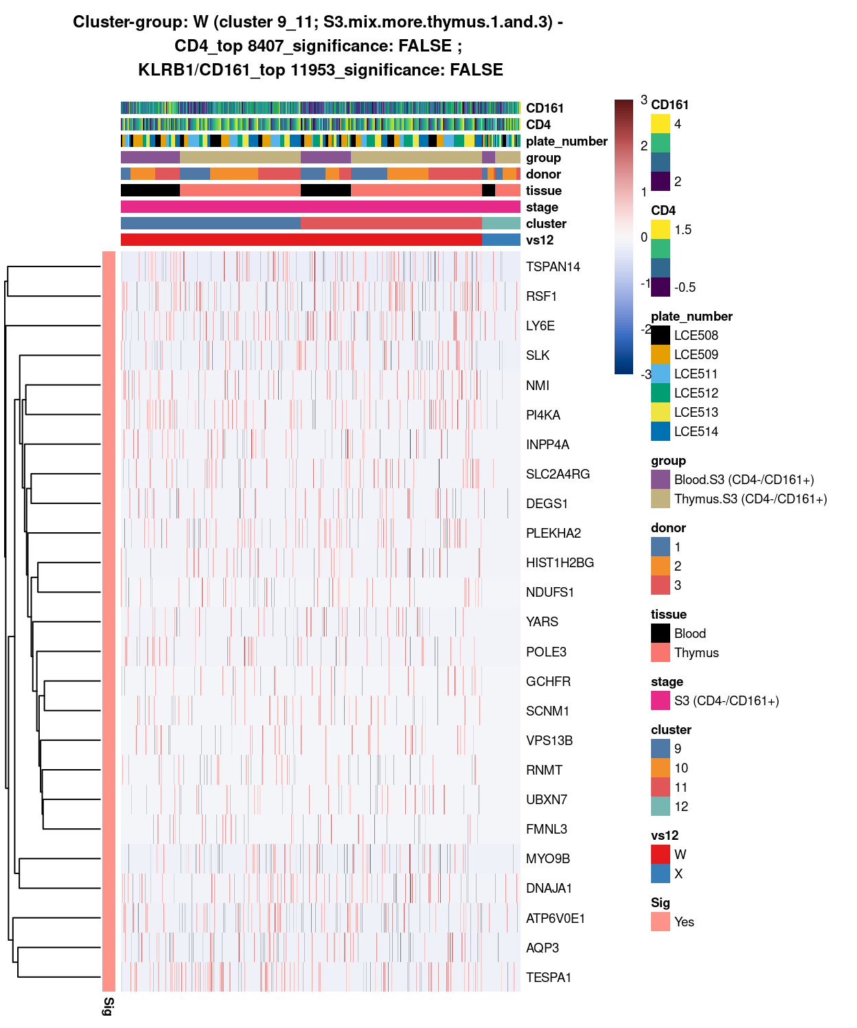
(#fig:heat-uniquely-up-logExp-cluster-9_11-vs-12)Heatmap of log-expression values in each sample for the top uniquely upregulated marker genes. Each column is a sample, each row a gene. Colours are capped at -3 and 3 to preserve dynamic range. Ranking of CD4 and CD161/KLRB1 from top of the DGE list sorted in ascending order of FDR and their statistical significance (TRUE = FDR < 0.05) are provided in the title.

Show code

##########################################################
# look at cluster-group X / cluster 12 (i.e.  S3.mix.more.thymus.4.center)
chosen <- "X"
X_uniquely_up <- vs12_uniquely_up[[chosen]]

# add description for the chosen cluster-group
x <- "(cluster 12; S3.mix.more.thymus.4.center)"

# look only at protein coding gene (pcg)
# NOTE: not suggest to narrow down into pcg as it remove all significant candidates (FDR << 0.05) !
# X_uniquely_up_pcg <- X_uniquely_up[intersect(protein_coding_gene_set, rownames(X_uniquely_up)), ]

# get rid of noise (i.e. pseudo, ribo, mito, sex) that collaborator not interested in
X_uniquely_up_noiseR <- X_uniquely_up[setdiff(rownames(X_uniquely_up), c(pseudogene_set, mito_set, ribo_set, sex_set)), ]

# see if key marker, "CD4 and/or ""KLRB1/CD161"", contain in the DE list + if it is "significant (i.e FDR <0.05)
y <- c("CD4",
       which(rownames(X_uniquely_up_noiseR) %in% "CD4"),
       X_uniquely_up_noiseR[which(rownames(X_uniquely_up_noiseR) %in% "CD4"), ]$FDR < 0.05)
z <- c("KLRB1/CD161",
       which(rownames(X_uniquely_up_noiseR) %in% "KLRB1"),
       X_uniquely_up_noiseR[which(rownames(X_uniquely_up_noiseR) %in% "KLRB1"), ]$FDR < 0.05)

# top25 only + gene-of-interest
best_set <- X_uniquely_up_noiseR[1:25, ]

Show code

# heatmap
plotHeatmap(
  cp,
  features = rownames(best_set),
  columns = order(
    cp$vs12,
    cp$cluster,
    cp$stage,
    cp$tissue,
    cp$donor,
    cp$group,
    cp$plate_number,
    cp$CD4,
    cp$CD161),
  colour_columns_by = c(
    "vs12",
    "cluster",
    "stage",
    "tissue",
    "donor",
    "group",
    "plate_number",
    "CD4",
    "CD161"),
  cluster_cols = FALSE,
  center = TRUE,
  symmetric = TRUE,
  zlim = c(-3, 3),
  show_colnames = FALSE,
  # annotation_row = data.frame(
  #   Sig = factor(
  #     ifelse(best_set[, "FDR"] < 0.05, "Yes", "No"),
  #     # TODO: temp trick to deal with the row-colouring problem
  #     # levels = c("Yes", "No")),
  #     levels = c("Yes")),
  #   row.names = rownames(best_set)),
  main = paste0("Cluster-group: ", chosen, " ", x, " - \n",
                y[1], "_top ", y[2], "_significance: ", y[3], " ; \n",
                z[1], "_top ", z[2], "_significance: ", z[3]),
  column_annotation_colors = list(
    # Sig = c("Yes" = "red", "No" = "lightgrey"),
    vs12 = vs12_colours,
    cluster = cluster_colours,
    stage = stage_colours,
    tissue = tissue_colours,
    donor = donor_colours,
    group = group_colours,
    plate_number = plate_number_colours),
  color = hcl.colors(101, "Blue-Red 3"),
  fontsize = 7)

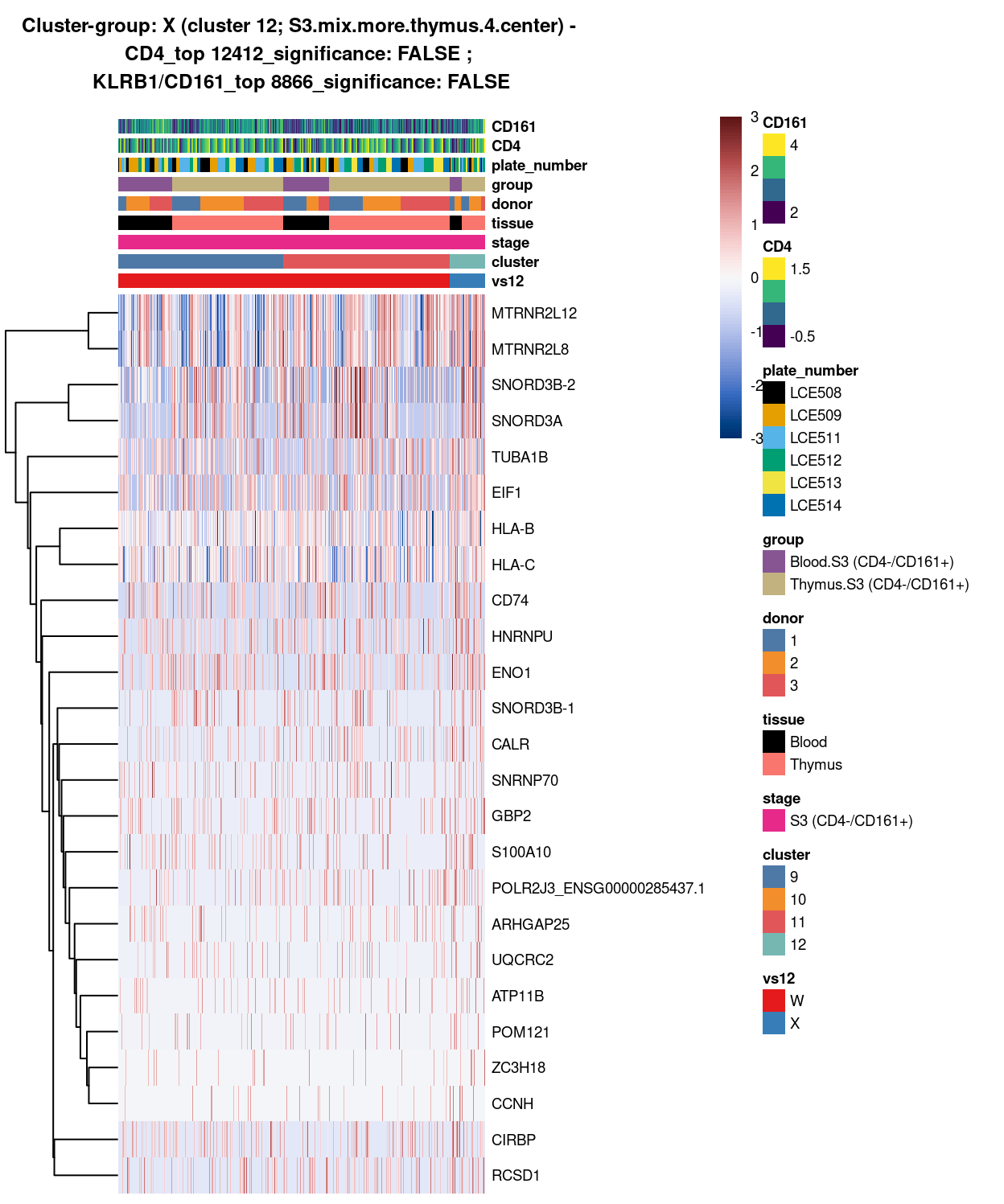
(#fig:heat-uniquely-up-logExp-cluster-12-vs-9_11)Heatmap of log-expression values in each sample for the top uniquely upregulated marker genes. Each column is a sample, each row a gene. Colours are capped at -3 and 3 to preserve dynamic range. Ranking of CD4 and CD161/KLRB1 from top of the DGE list sorted in ascending order of FDR and their statistical significance (TRUE = FDR < 0.05) are provided in the title.

DGE lists of these comparisons are available in output/marker_genes/S3_only/uniquely_up/cluster_9_11_vs_12/.

SUMMARY: 9_11 vs 12 (W vs X)

• cluster 9_11 (S3.mix.more.thymus.1.and.3 >>> lots of marker more frequently expressed in 9_11
• cluster 12 (S3.mix.more.thymus.4 >>> no statistically significant markers
• COMMENT: consistently, 12 show no marker, uniqueness is from cluster 9_11

cluster_9_10_11_vs_cluster_12

Show code

#########
# Y vs Z
#########

##########################################################################################
# cluster 9_10_11 (i.e. S3.mix.more.thymus.1.and.2.and.3) vs cluster 12 (i.e. S3.mix.more.thymus.4.center)

# checkpoint
cp <- sce

# classify cluster-group for comparison
cp$vs13 <- factor(ifelse(cp$cluster == 9 | cp$cluster == 10 | cp$cluster == 11, "Y", "Z"))

# set vs colours
vs13_colours <- setNames(
  palette.colors(nlevels(cp$vs13), "Set1"),
  levels(cp$vs13))
cp$colours$vs13_colours <- vs13_colours[cp$vs13]

# find unique DE ./. cluster-groups
vs13_uniquely_up <- findMarkers(
  cp,
  groups = cp$vs13,
  block = cp$block,
  pval.type = "all",
  direction = "up")

# export DGE lists
saveRDS(
  vs13_uniquely_up,
  here("data", "marker_genes", "S3_only", "C094_Pellicci.uniquely_up.cluster_9_10_11_vs_12.rds"),
  compress = "xz")

dir.create(here("output", "marker_genes", "S3_only", "uniquely_up", "cluster_9_10_11_vs_12"), recursive = TRUE)

vs_pair <- c("9_10_11", "12")

message("Writing 'uniquely_up (cluster_9_10_11_vs_12)' marker genes to file.")
for (n in names(vs13_uniquely_up)) {
  message(n)
  gzout <- gzfile(
    description = here(
      "output",
      "marker_genes",
      "S3_only",
      "uniquely_up",
      "cluster_9_10_11_vs_12",
      paste0("cluster_",
             vs_pair[which(names(vs13_uniquely_up) %in% n)],
             "_vs_",
             vs_pair[-which(names(vs13_uniquely_up) %in% n)][1],
             ".uniquely_up.csv.gz")),
    open = "wb")
  write.table(
    x = vs13_uniquely_up[[n]] %>%
      as.data.frame() %>%
      tibble::rownames_to_column("gene_ID"),
    file = gzout,
    sep = ",",
    quote = FALSE,
    row.names = FALSE,
    col.names = TRUE)
  close(gzout)
}

Show code

###############################################################
# look at cluster-group Y / cluster 9_10_11 (i.e. S3.mix.more.thymus.1.and.2.and.3)
chosen <- "Y"
Y_uniquely_up <- vs13_uniquely_up[[chosen]]

# add description for the chosen cluster-group
x <- "(cluster 9_10_11; S3.mix.more.thymus.1.and.2.and.3)"

# look only at protein coding gene (pcg)
# NOTE: not suggest to narrow down into pcg as it remove all significant candidates (FDR << 0.05) !
# Y_uniquely_up_pcg <- Y_uniquely_up[intersect(protein_coding_gene_set, rownames(Y_uniquely_up)), ]

# get rid of noise (i.e. pseudo, ribo, mito, sex) that collaborator not interested in
Y_uniquely_up_noiseR <- Y_uniquely_up[setdiff(rownames(Y_uniquely_up), c(pseudogene_set, mito_set, ribo_set, sex_set)), ]

# see if key marker, "CD4 and/or ""KLRB1/CD161"", contain in the DE list + if it is "significant (i.e FDR <0.05)
y <- c("CD4",
       which(rownames(Y_uniquely_up_noiseR) %in% "CD4"),
       Y_uniquely_up_noiseR[which(rownames(Y_uniquely_up_noiseR) %in% "CD4"), ]$FDR < 0.05)
z <- c("KLRB1/CD161",
       which(rownames(Y_uniquely_up_noiseR) %in% "KLRB1"),
       Y_uniquely_up_noiseR[which(rownames(Y_uniquely_up_noiseR) %in% "KLRB1"), ]$FDR < 0.05)

# top25 only + gene-of-interest
best_set <- Y_uniquely_up_noiseR[1:25, ]

Show code

# heatmap
plotHeatmap(
  cp,
  features = rownames(best_set),
  columns = order(
    cp$vs13,
    cp$cluster,
    cp$stage,
    cp$tissue,
    cp$donor,
    cp$group,
    cp$plate_number,
    cp$CD4,
    cp$CD161),
  colour_columns_by = c(
    "vs13",
    "cluster",
    "stage",
    "tissue",
    "donor",
    "group",
    "plate_number",
    "CD4",
    "CD161"),
  cluster_cols = FALSE,
  center = TRUE,
  symmetric = TRUE,
  zlim = c(-3, 3),
  show_colnames = FALSE,
  annotation_row = data.frame(
    Sig = factor(
      ifelse(best_set[, "FDR"] < 0.05, "Yes", "No"),
      # TODO: temp trick to deal with the row-colouring problem
      # levels = c("Yes", "No")),
      levels = c("Yes")),
    row.names = rownames(best_set)),
  main = paste0("Cluster-group: ", chosen, " ", x, " - \n",
                y[1], "_top ", y[2], "_significance: ", y[3], " ; \n",
                z[1], "_top ", z[2], "_significance: ", z[3]),
  column_annotation_colors = list(
    # Sig = c("Yes" = "red", "No" = "lightgrey"),
    vs13 = vs13_colours,
    cluster = cluster_colours,
    stage = stage_colours,
    tissue = tissue_colours,
    donor = donor_colours,
    group = group_colours,
    plate_number = plate_number_colours),
  color = hcl.colors(101, "Blue-Red 3"),
  fontsize = 7)

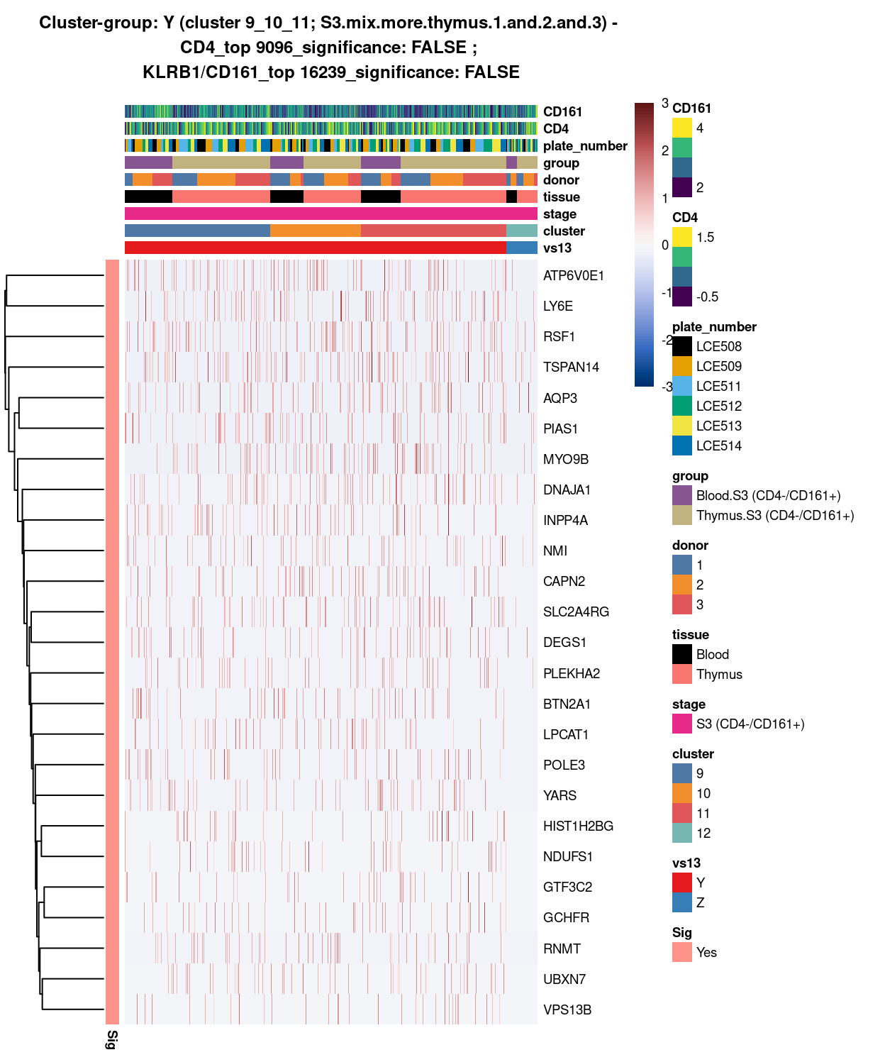
(#fig:heat-uniquely-up-logExp-cluster-9_10_11-vs-12)Heatmap of log-expression values in each sample for the top uniquely upregulated marker genes. Each column is a sample, each row a gene. Colours are capped at -3 and 3 to preserve dynamic range. Ranking of CD4 and CD161/KLRB1 from top of the DGE list sorted in ascending order of FDR and their statistical significance (TRUE = FDR < 0.05) are provided in the title.

Show code

##########################################################
# look at cluster-group Z / cluster 12 (i.e. S3.mix.more.thymus.4.center)
chosen <- "Z"
Z_uniquely_up <- vs13_uniquely_up[[chosen]]

# add description for the chosen cluster-group
x <- "(cluster 12; S3.mix.more.thymus.4.center)"

# look only at protein coding gene (pcg)
# NOTE: not suggest to narrow down into pcg as it remove all significant candidates (FDR << 0.05) !
# Z_uniquely_up_pcg <- Z_uniquely_up[intersect(protein_coding_gene_set, rownames(Z_uniquely_up)), ]

# get rid of noise (i.e. pseudo, ribo, mito, sex) that collaborator not interested in
Z_uniquely_up_noiseR <- Z_uniquely_up[setdiff(rownames(Z_uniquely_up), c(pseudogene_set, mito_set, ribo_set, sex_set)), ]

# see if key marker, "CD4 and/or ""KLRB1/CD161"", contain in the DE list + if it is "significant (i.e FDR <0.05)
y <- c("CD4",
       which(rownames(Z_uniquely_up_noiseR) %in% "CD4"),
       Z_uniquely_up_noiseR[which(rownames(Z_uniquely_up_noiseR) %in% "CD4"), ]$FDR < 0.05)
z <- c("KLRB1/CD161",
       which(rownames(Z_uniquely_up_noiseR) %in% "KLRB1"),
       Z_uniquely_up_noiseR[which(rownames(Z_uniquely_up_noiseR) %in% "KLRB1"), ]$FDR < 0.05)

# top25 only + gene-of-interest
best_set <- Z_uniquely_up_noiseR[1:25, ]

Show code

# heatmap
plotHeatmap(
  cp,
  features = rownames(best_set),
  columns = order(
    cp$vs13,
    cp$cluster,
    cp$stage,
    cp$tissue,
    cp$donor,
    cp$group,
    cp$plate_number,
    cp$CD4,
    cp$CD161),
  colour_columns_by = c(
    "vs13",
    "cluster",
    "stage",
    "tissue",
    "donor",
    "group",
    "plate_number",
    "CD4",
    "CD161"),
  cluster_cols = FALSE,
  center = TRUE,
  symmetric = TRUE,
  zlim = c(-3, 3),
  show_colnames = FALSE,
  # annotation_row = data.frame(
  #   Sig = factor(
  #     ifelse(best_set[, "FDR"] < 0.05, "Yes", "No"),
  #     # TODO: temp trick to deal with the row-colouring problem
  #     # levels = c("Yes", "No")),
  #     levels = c("Yes")),
  #   row.names = rownames(best_set)),
  main = paste0("Cluster-group: ", chosen, " ", x, " - \n",
                y[1], "_top ", y[2], "_significance: ", y[3], " ; \n",
                z[1], "_top ", z[2], "_significance: ", z[3]),
  column_annotation_colors = list(
    # Sig = c("Yes" = "red", "No" = "lightgrey"),
    vs13 = vs13_colours,
    cluster = cluster_colours,
    stage = stage_colours,
    tissue = tissue_colours,
    donor = donor_colours,
    group = group_colours,
    plate_number = plate_number_colours),
  color = hcl.colors(101, "Blue-Red 3"),
  fontsize = 7)

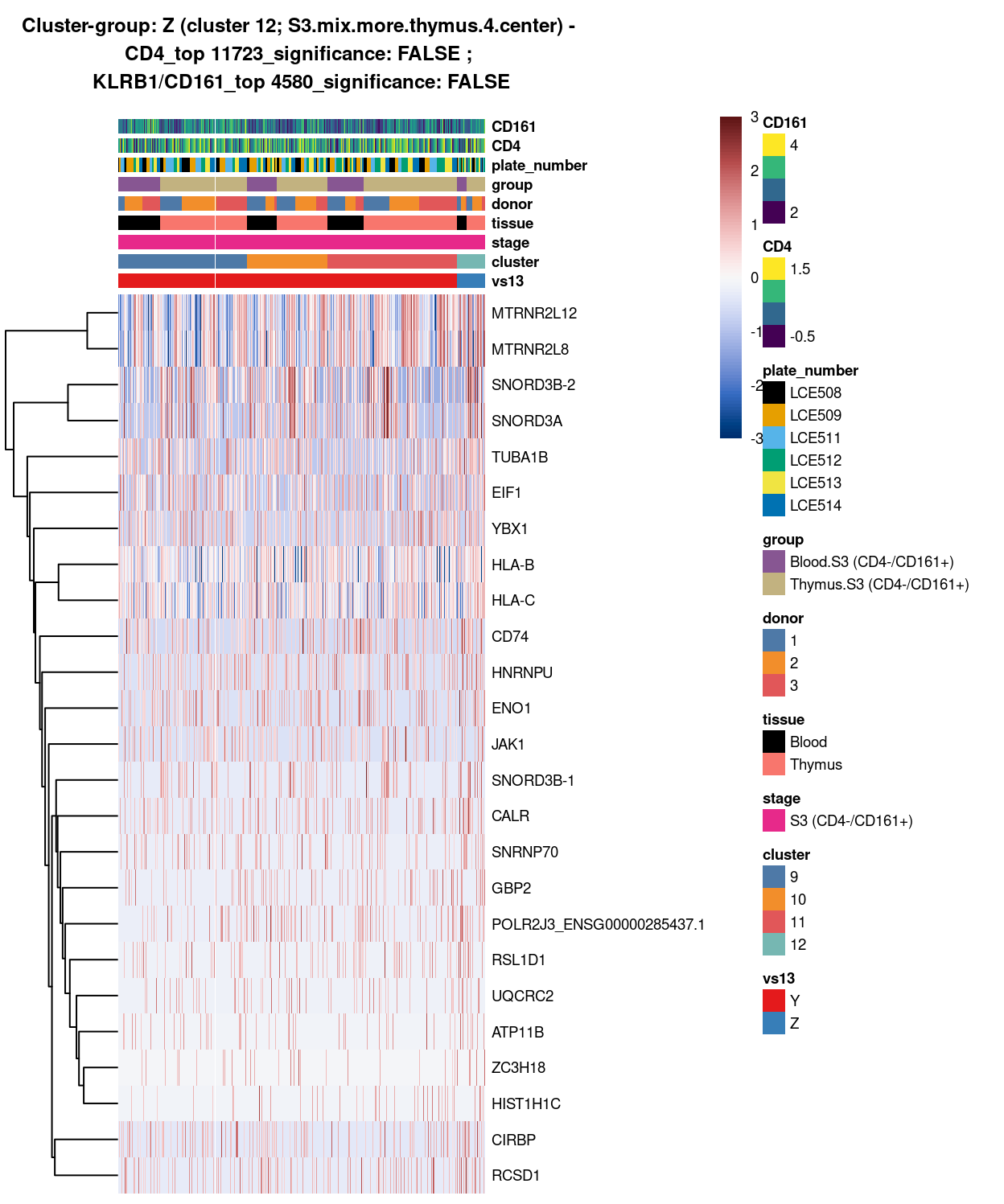
(#fig:heat-uniquely-up-logExp-cluster-12-vs-9_10_11)Heatmap of log-expression values in each sample for the top uniquely upregulated marker genes. Each column is a sample, each row a gene. Colours are capped at -3 and 3 to preserve dynamic range. Ranking of CD4 and CD161/KLRB1 from top of the DGE list sorted in ascending order of FDR and their statistical significance (TRUE = FDR < 0.05) are provided in the title.

DGE lists of these comparisons are available in output/marker_genes/S3_only/uniquely_up/cluster_9_10_11_vs_12/.

SUMMARY: 9_10_11 vs 12 (Y vs Z)

• cluster 9_10_11 (S3.mix.more.thymus.1.and.2.and.3 >>> lots of marker more frequently expressed in 9_10_11
• cluster 12 (i.e. S3.mix.more.thymus.4 >>> no statistically significant marker found
• COMMENT: consistently, cluster 12 shows no marker, uniqueness is coming from cluster 9_10_11

Selected pairwise comparisons - integrated

To have a comprehensive overview, the above analyses were summarized in the following heatmap per cluster:

Show code

# NOTE: The following is a workaround to the lack of support for tabsets in 
#       distill (see https://github.com/rstudio/distill/issues/11 and 
#       https://github.com/rstudio/distill/issues/11#issuecomment-692142414 in 
#       particular).
xaringanExtra::use_panelset()

Cluster_9_integrated

Show code

############
# cluster 9
############

chosen <- "9"
# add description for the chosen cluster-group
x <- "(S3.mix.more.thymus.1)"
# retain only significant markers (FDR<0.05) + keep only required output columns
A_uniquely_up_noiseR_sig <- A_uniquely_up_noiseR[A_uniquely_up_noiseR$FDR<0.05,][ ,c(1:3)]
C_uniquely_up_noiseR_sig <- C_uniquely_up_noiseR[C_uniquely_up_noiseR$FDR<0.05,][ ,c(1:3)]
E_uniquely_up_noiseR_sig <- E_uniquely_up_noiseR[E_uniquely_up_noiseR$FDR<0.05,][ ,c(1:3)]
P_uniquely_up_noiseR_sig <- P_uniquely_up_noiseR[P_uniquely_up_noiseR$FDR<0.05,][ ,c(1:3)]
cluster9_uniquely_up_noiseR_sig <- cluster9_uniquely_up_noiseR[cluster9_uniquely_up_noiseR$FDR<0.05,][ ,c(1:3)]
# add top column
A_uniquely_up_noiseR_sig$top <- 1:nrow(A_uniquely_up_noiseR_sig)
C_uniquely_up_noiseR_sig$top <- 1:nrow(C_uniquely_up_noiseR_sig)
E_uniquely_up_noiseR_sig$top <- 1:nrow(E_uniquely_up_noiseR_sig)
P_uniquely_up_noiseR_sig$top <- 1:nrow(P_uniquely_up_noiseR_sig)
cluster9_uniquely_up_noiseR_sig$top <- 1:nrow(cluster9_uniquely_up_noiseR_sig)
# unify S4 objects, sort by top (ascending) then FDR (ascending), keep only first unique entry for each marker
ACEP9_uniquely_up_noiseR_sig <- rbind2(A_uniquely_up_noiseR_sig,
                                       C_uniquely_up_noiseR_sig,
                                       E_uniquely_up_noiseR_sig,
                                       P_uniquely_up_noiseR_sig,
                                       cluster9_uniquely_up_noiseR_sig)
ACEP9_uniquely_up_noiseR_sig_sort <- ACEP9_uniquely_up_noiseR_sig[with(ACEP9_uniquely_up_noiseR_sig, order(top, FDR)), ]
ACEP9_uniquely_up_noiseR_sig_sort_uniq <- ACEP9_uniquely_up_noiseR_sig_sort[unique(rownames(ACEP9_uniquely_up_noiseR_sig_sort)), ]
# # de-select unannotated/ not well-characterised genes
# deselected <- c("NPIPB13", "NPIPB3", "NPIPB11", "NPIPB5", "NPIPB4", "EEF1A1", "ACTG1", "ACTB", "IFITM1")
deselected <- c("MALAT1", "MTRNR2L12", "MTRNR2L8")
ACEP9_uniquely_up_noiseR_sig_sort_uniq_selected <- ACEP9_uniquely_up_noiseR_sig_sort_uniq[!(rownames(ACEP9_uniquely_up_noiseR_sig_sort_uniq) %in% deselected), ]

# export DGE lists
saveRDS(
  ACEP9_uniquely_up_noiseR_sig_sort_uniq_selected,
  here("data", "marker_genes", "S3_only", "C094_Pellicci.uniquely_up.cluster_9_integrated.rds"),
  compress = "xz")
dir.create(here("output", "marker_genes", "S3_only", "uniquely_up", "integrated"), recursive = TRUE)
message("Writing 'uniquely_up (cluster_9_integrated)' marker genes to file.")
gzout <- gzfile(
  description = here(
    "output",
    "marker_genes",
    "S3_only",
    "uniquely_up",
    "integrated",
    paste0("cluster_9_integrated",
           ".uniquely_up.csv.gz")),
  open = "wb")
write.table(
  x = ACEP9_uniquely_up_noiseR_sig_sort_uniq_selected %>%
    as.data.frame() %>%
    tibble::rownames_to_column("gene_ID"),
  file = gzout,
  sep = ",",
  quote = FALSE,
  row.names = FALSE,
  col.names = TRUE)
close(gzout)
# top only + gene-of-interest
best_set <- ACEP9_uniquely_up_noiseR_sig_sort_uniq_selected[1:50, ]

Show code

# heatmap
plotHeatmap(
  sce,
  features = rownames(best_set),
  columns = order(
    sce$cluster,
    sce$stage,
    sce$tissue,
    sce$donor,
    sce$group,
    sce$plate_number,
    sce$CD4,
    sce$CD161),
  colour_columns_by = c(
    "cluster",
    "stage",
    "tissue",
    "donor",
    "group",
    "plate_number",
    "CD4",
    "CD161"),
  cluster_cols = FALSE,
  center = TRUE,
  symmetric = TRUE,
  zlim = c(-3, 3),
  show_colnames = FALSE,
  annotation_row = data.frame(
    # TODO: temp trick to deal with the row-colouring problem
    cluster9.vs.10 = factor(ifelse(rownames(best_set) %in% rownames(A_uniquely_up_noiseR_sig), "DE", "not DE"), levels = c("DE")),
    cluster9.vs.11 = factor(ifelse(rownames(best_set) %in% rownames(C_uniquely_up_noiseR_sig), "DE", "not DE"), levels = c("DE")),
    cluster9.vs.12 = factor(ifelse(rownames(best_set) %in% rownames(E_uniquely_up_noiseR_sig), "DE", "not DE"), levels = c("DE")),
    cluster9.vs.10_11 = factor(ifelse(rownames(best_set) %in% rownames(P_uniquely_up_noiseR_sig), "DE", "not DE"), levels = c("DE")),
    cluster9.vs.10.vs.11.VS.12 = factor(ifelse(rownames(best_set) %in% rownames(cluster9_uniquely_up_noiseR_sig), "DE", "not DE"), levels = c("DE")),    
    row.names = rownames(best_set)),
  main = paste0("Cluster ", chosen, " ", x),
  column_annotation_colors = list(
    # Sig = c("Yes" = "red", "No" = "lightgrey"),
    cluster = cluster_colours,
    stage = stage_colours,
    tissue = tissue_colours,
    donor = donor_colours,
    group = group_colours,
    plate_number = plate_number_colours),
  color = hcl.colors(101, "Blue-Red 3"),
  fontsize = 7)

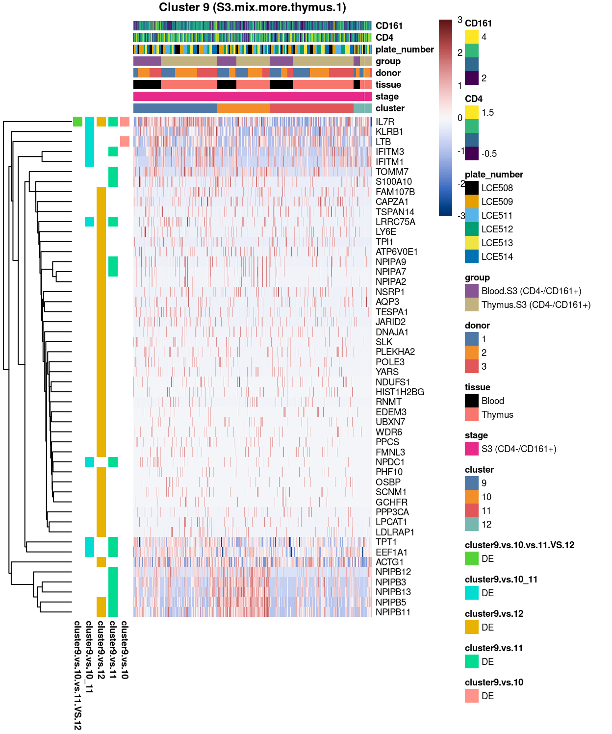
Figure 19: Heatmap of log-expression values in each sample for the top uniquely upregulated marker genes. Each column is a sample, each row a gene. Colours are capped at -3 and 3 to preserve dynamic range.

Cluster_10_integrated

Show code

############
# cluster 10
############

chosen <- "10"
# add description for the chosen cluster-group
x <- "(S3.mix.more.thymus.2)"
# retain only significant markers (FDR<0.05) + keep only required output columns
B_uniquely_up_noiseR_sig <- B_uniquely_up_noiseR[B_uniquely_up_noiseR$FDR<0.05,][ ,c(1:3)]
G_uniquely_up_noiseR_sig <- G_uniquely_up_noiseR[G_uniquely_up_noiseR$FDR<0.05,][ ,c(1:3)]
I_uniquely_up_noiseR_sig <- I_uniquely_up_noiseR[I_uniquely_up_noiseR$FDR<0.05,][ ,c(1:3)]
R_uniquely_up_noiseR_sig <- R_uniquely_up_noiseR[R_uniquely_up_noiseR$FDR<0.05,][ ,c(1:3)]
cluster10_uniquely_up_noiseR_sig <- cluster10_uniquely_up_noiseR[cluster10_uniquely_up_noiseR$FDR<0.05,][ ,c(1:3)]
# add top column
B_uniquely_up_noiseR_sig$top <- 1:nrow(B_uniquely_up_noiseR_sig)
G_uniquely_up_noiseR_sig$top <- 1:nrow(G_uniquely_up_noiseR_sig)
I_uniquely_up_noiseR_sig$top <- 1:nrow(I_uniquely_up_noiseR_sig)
R_uniquely_up_noiseR_sig$top <- 1:nrow(R_uniquely_up_noiseR_sig)
cluster10_uniquely_up_noiseR_sig$top <- 1:nrow(cluster10_uniquely_up_noiseR_sig)
# unify S4 objects, sort by top (ascending) then FDR (ascending), keep only first unique entry for each marker
BGIR10_uniquely_up_noiseR_sig <- rbind2(B_uniquely_up_noiseR_sig,
                                        G_uniquely_up_noiseR_sig,
                                        I_uniquely_up_noiseR_sig,
                                        R_uniquely_up_noiseR_sig,
                                        cluster10_uniquely_up_noiseR_sig)
BGIR10_uniquely_up_noiseR_sig_sort <- BGIR10_uniquely_up_noiseR_sig[with(BGIR10_uniquely_up_noiseR_sig, order(top, FDR)), ]
BGIR10_uniquely_up_noiseR_sig_sort_uniq <- BGIR10_uniquely_up_noiseR_sig_sort[unique(rownames(BGIR10_uniquely_up_noiseR_sig_sort)), ]
# # de-select unannotated/ not well-characterised genes
# deselected <- c("NPIPB13", "NPIPB3", "NPIPB11", "NPIPB5", "NPIPB4", "EEF1A1", "ACTG1", "ACTB", "IFITM1")
deselected <- c("MALAT1", "MTRNR2L12", "MTRNR2L8")
BGIR10_uniquely_up_noiseR_sig_sort_uniq_selected <- BGIR10_uniquely_up_noiseR_sig_sort_uniq[!(rownames(BGIR10_uniquely_up_noiseR_sig_sort_uniq) %in% deselected), ]

# export DGE lists
saveRDS(
  BGIR10_uniquely_up_noiseR_sig_sort_uniq_selected,
  here("data", "marker_genes", "S3_only", "C094_Pellicci.uniquely_up.cluster_10_integrated.rds"),
  compress = "xz")
dir.create(here("output", "marker_genes", "S3_only", "uniquely_up", "integrated"), recursive = TRUE)
message("Writing 'uniquely_up (cluster_10_integrated)' marker genes to file.")
gzout <- gzfile(
  description = here(
    "output",
    "marker_genes",
    "S3_only",
    "uniquely_up",
    "integrated",
    paste0("cluster_10_integrated",
           ".uniquely_up.csv.gz")),
  open = "wb")
write.table(
  x = BGIR10_uniquely_up_noiseR_sig_sort_uniq_selected %>%
    as.data.frame() %>%
    tibble::rownames_to_column("gene_ID"),
  file = gzout,
  sep = ",",
  quote = FALSE,
  row.names = FALSE,
  col.names = TRUE)
close(gzout)
# top only + gene-of-interest
# best_set <- BGIR10_uniquely_up_noiseR_sig_sort_uniq_selected[1:50, ]
# NOTE: have 28 markers only
best_set <- BGIR10_uniquely_up_noiseR_sig_sort_uniq_selected[1:28, ]

Show code

# heatmap
plotHeatmap(
  sce,
  features = rownames(best_set),
  columns = order(
    sce$cluster,
    sce$stage,
    sce$tissue,
    sce$donor,
    sce$group,
    sce$plate_number,
    sce$CD4,
    sce$CD161),
  colour_columns_by = c(
    "cluster",
    "stage",
    "tissue",
    "donor",
    "group",
    "plate_number",
    "CD4",
    "CD161"),
  cluster_cols = FALSE,
  center = TRUE,
  symmetric = TRUE,
  zlim = c(-3, 3),
  show_colnames = FALSE,
  annotation_row = data.frame(
    # TODO: temp trick to deal with the row-colouring problem
    cluster10.vs.9 = factor(ifelse(rownames(best_set) %in% rownames(B_uniquely_up_noiseR_sig), "DE", "not DE"), levels = c("DE")),
    cluster10.vs.11 = factor(ifelse(rownames(best_set) %in% rownames(G_uniquely_up_noiseR_sig), "DE", "not DE"), levels = c("DE")),
    cluster10.vs.12 = factor(ifelse(rownames(best_set) %in% rownames(I_uniquely_up_noiseR_sig), "DE", "not DE"), levels = c("DE")),
    cluster10.vs.9_11 = factor(ifelse(rownames(best_set) %in% rownames(R_uniquely_up_noiseR_sig), "DE", "not DE"), levels = c("DE")),
    cluster10.vs.9.vs.11.VS.12 = factor(ifelse(rownames(best_set) %in% rownames(cluster10_uniquely_up_noiseR_sig), "DE", "not DE"), levels = c("DE")),    
    row.names = rownames(best_set)),
  main = paste0("Cluster ", chosen, " ", x),
  column_annotation_colors = list(
    # Sig = c("Yes" = "red", "No" = "lightgrey"),
    cluster = cluster_colours,
    stage = stage_colours,
    tissue = tissue_colours,
    donor = donor_colours,
    group = group_colours,
    plate_number = plate_number_colours),
  color = hcl.colors(101, "Blue-Red 3"),
  fontsize = 7)

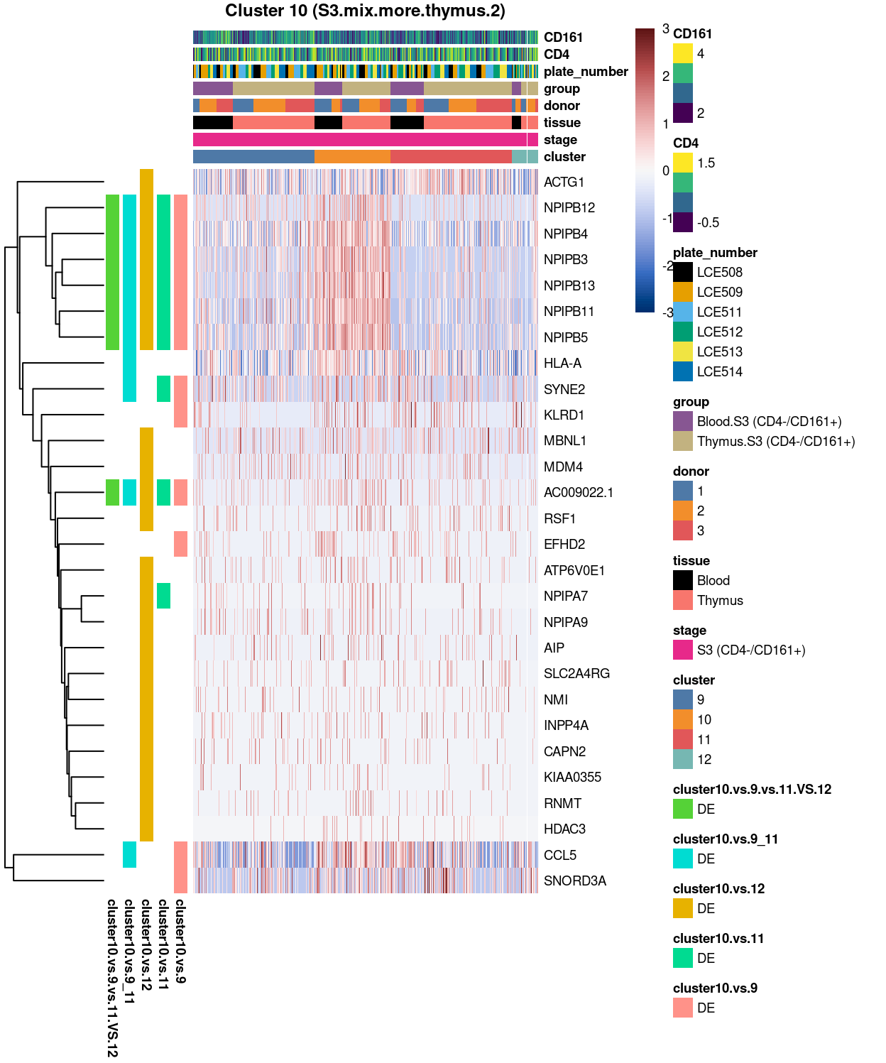
Figure 20: Heatmap of log-expression values in each sample for the top uniquely upregulated marker genes. Each column is a sample, each row a gene. Colours are capped at -3 and 3 to preserve dynamic range.

Cluster_11_integrated

Show code

############
# cluster 11
############

chosen <- "11"
# add description for the chosen cluster-group
x <- "(S3.mix.more.thymus.3)"
# retain only significant markers (FDR<0.05) + keep only required output columns
D_uniquely_up_noiseR_sig <- D_uniquely_up_noiseR[D_uniquely_up_noiseR$FDR<0.05,][ ,c(1:3)]
H_uniquely_up_noiseR_sig <- H_uniquely_up_noiseR[H_uniquely_up_noiseR$FDR<0.05,][ ,c(1:3)]
K_uniquely_up_noiseR_sig <- K_uniquely_up_noiseR[K_uniquely_up_noiseR$FDR<0.05,][ ,c(1:3)]
N_uniquely_up_noiseR_sig <- N_uniquely_up_noiseR[N_uniquely_up_noiseR$FDR<0.05,][ ,c(1:3)]
cluster11_uniquely_up_noiseR_sig <- cluster11_uniquely_up_noiseR[cluster11_uniquely_up_noiseR$FDR<0.05,][ ,c(1:3)]
# add top column
D_uniquely_up_noiseR_sig$top <- 1:nrow(D_uniquely_up_noiseR_sig)
K_uniquely_up_noiseR_sig$top <- 1:nrow(K_uniquely_up_noiseR_sig)
# TODO: fix error - exclude list from rbind2 if empty
# H_uniquely_up_noiseR_sig$top <- 1:nrow(H_uniquely_up_noiseR_sig)
# N_uniquely_up_noiseR_sig$top <- 1:nrow(N_uniquely_up_noiseR_sig)
# cluster11_uniquely_up_noiseR_sig$top <- 1:nrow(cluster11_uniquely_up_noiseR_sig)
# unify S4 objects, sort by top (ascending) then FDR (ascending), keep only first unique entry for each marker
DHKN11_uniquely_up_noiseR_sig <- rbind2(D_uniquely_up_noiseR_sig,
                                        H_uniquely_up_noiseR_sig,
                                        K_uniquely_up_noiseR_sig,
                                        N_uniquely_up_noiseR_sig,
                                        cluster11_uniquely_up_noiseR_sig)
DHKN11_uniquely_up_noiseR_sig_sort <- DHKN11_uniquely_up_noiseR_sig[with(DHKN11_uniquely_up_noiseR_sig, order(top, FDR)), ]
DHKN11_uniquely_up_noiseR_sig_sort_uniq <- DHKN11_uniquely_up_noiseR_sig_sort[unique(rownames(DHKN11_uniquely_up_noiseR_sig_sort)), ]
# # de-select unannotated/ not well-characterised genes
# deselected <- c("NPIPB13", "NPIPB3", "NPIPB11", "NPIPB5", "NPIPB4", "EEF1A1", "ACTG1", "ACTB", "IFITM1")
deselected <- c("MALAT1", "MTRNR2L12", "MTRNR2L8")
DHKN11_uniquely_up_noiseR_sig_sort_uniq_selected <- DHKN11_uniquely_up_noiseR_sig_sort_uniq[!(rownames(DHKN11_uniquely_up_noiseR_sig_sort_uniq) %in% deselected), ]

# export DGE lists
saveRDS(
  DHKN11_uniquely_up_noiseR_sig_sort_uniq_selected,
  here("data", "marker_genes", "S3_only", "C094_Pellicci.uniquely_up.cluster_11_integrated.rds"),
  compress = "xz")
dir.create(here("output", "marker_genes", "S3_only", "uniquely_up", "integrated"), recursive = TRUE)
message("Writing 'uniquely_up (cluster_11_integrated)' marker genes to file.")
gzout <- gzfile(
  description = here(
    "output",
    "marker_genes",
    "S3_only",
    "uniquely_up",
    "integrated",
    paste0("cluster_11_integrated",
           ".uniquely_up.csv.gz")),
  open = "wb")
write.table(
  x = DHKN11_uniquely_up_noiseR_sig_sort_uniq_selected %>%
    as.data.frame() %>%
    tibble::rownames_to_column("gene_ID"),
  file = gzout,
  sep = ",",
  quote = FALSE,
  row.names = FALSE,
  col.names = TRUE)
close(gzout)
# top only + gene-of-interest
best_set <- DHKN11_uniquely_up_noiseR_sig_sort_uniq_selected[1:50, ]

Show code

# heatmap
plotHeatmap(
  sce,
  features = rownames(best_set),
  columns = order(
    sce$cluster,
    sce$stage,
    sce$tissue,
    sce$donor,
    sce$group,
    sce$plate_number,
    sce$CD4,
    sce$CD161),
  colour_columns_by = c(
    "cluster",
    "stage",
    "tissue",
    "donor",
    "group",
    "plate_number",
    "CD4",
    "CD161"),
  cluster_cols = FALSE,
  center = TRUE,
  symmetric = TRUE,
  zlim = c(-3, 3),
  show_colnames = FALSE,
  annotation_row = data.frame(
    # TODO: temp trick to deal with the row-colouring problem
    cluster11.vs.9 = factor(ifelse(rownames(best_set) %in% rownames(D_uniquely_up_noiseR_sig), "DE", "not DE"), levels = c("DE")),
    cluster11.vs.12 = factor(ifelse(rownames(best_set) %in% rownames(K_uniquely_up_noiseR_sig), "DE", "not DE"), levels = c("DE")),
    # TODO: work out how to remove `fill` from `not_DE`
    # cluster11.vs.10 = factor(ifelse(rownames(best_set) %in% rownames(H_uniquely_up_noiseR_sig), "DE", "not DE"), levels = c("DE")),
    # cluster11.vs.9_10 = factor(ifelse(rownames(best_set) %in% rownames(N_uniquely_up_noiseR_sig), "DE", "not DE"), levels = c("DE")),
    # cluster11.vs.9.vs.10.VS.12 = factor(ifelse(rownames(best_set) %in% rownames(cluster11_uniquely_up_noiseR_sig), "DE", "not DE"), levels = c("DE")),    
    row.names = rownames(best_set)),
  main = paste0("Cluster ", chosen, " ", x),
  column_annotation_colors = list(
    # Sig = c("Yes" = "red", "No" = "lightgrey"),
    cluster = cluster_colours,
    stage = stage_colours,
    tissue = tissue_colours,
    donor = donor_colours,
    group = group_colours,
    plate_number = plate_number_colours),
  color = hcl.colors(101, "Blue-Red 3"),
  fontsize = 7)

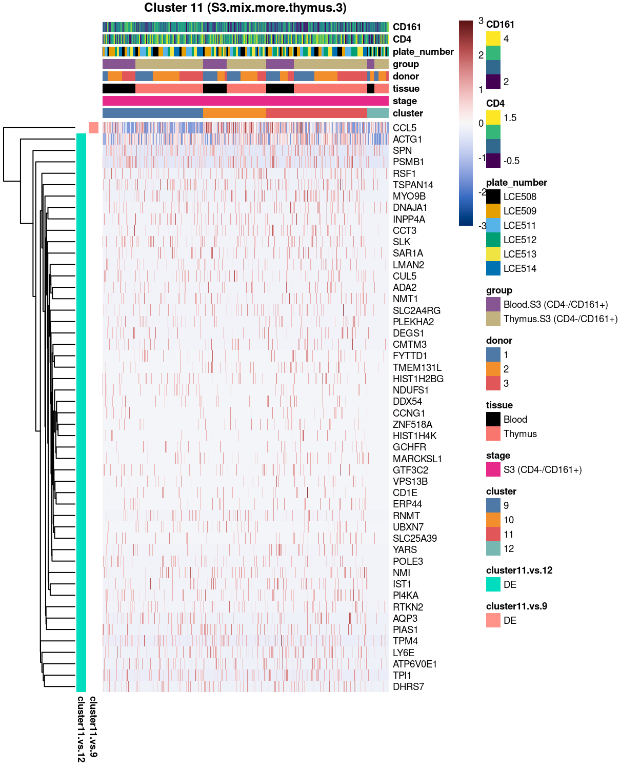
Figure 21: Heatmap of log-expression values in each sample for the top uniquely upregulated marker genes. Each column is a sample, each row a gene. Colours are capped at -3 and 3 to preserve dynamic range.

Cluster_12_integrated

Show code

############
# cluster 12
############

chosen <- "12"
# add description for the chosen cluster-group
x <- "(S3.mix.more.thymus.4.center)"
# retain only significant markers (FDR<0.05) + keep only required output columns
# F_uniquely_up_noiseR_sig <- F_uniquely_up_noiseR[F_uniquely_up_noiseR$FDR<0.05,][ ,c(1:3)]
# J_uniquely_up_noiseR_sig <- J_uniquely_up_noiseR[J_uniquely_up_noiseR$FDR<0.05,][ ,c(1:3)]
# L_uniquely_up_noiseR_sig <- L_uniquely_up_noiseR[L_uniquely_up_noiseR$FDR<0.05,][ ,c(1:3)]
# T_uniquely_up_noiseR_sig <- T_uniquely_up_noiseR[T_uniquely_up_noiseR$FDR<0.05,][ ,c(1:3)]
# V_uniquely_up_noiseR_sig <- V_uniquely_up_noiseR[V_uniquely_up_noiseR$FDR<0.05,][ ,c(1:3)]
# X_uniquely_up_noiseR_sig <- X_uniquely_up_noiseR[X_uniquely_up_noiseR$FDR<0.05,][ ,c(1:3)]
# Z_uniquely_up_noiseR_sig <- Z_uniquely_up_noiseR[Z_uniquely_up_noiseR$FDR<0.05,][ ,c(1:3)]
# cluster12_uniquely_up_noiseR_sig <- cluster12_uniquely_up_noiseR[cluster12_uniquely_up_noiseR$FDR<0.05,][ ,c(1:3)]
# NOTE: none of them are significantly different, thus needed an alternative path to make the plot
F_uniquely_up_noiseR_sig <- F_uniquely_up_noiseR[F_uniquely_up_noiseR$FDR<1,][ ,c(1:3)]
J_uniquely_up_noiseR_sig <- J_uniquely_up_noiseR[J_uniquely_up_noiseR$FDR<1,][ ,c(1:3)]
L_uniquely_up_noiseR_sig <- L_uniquely_up_noiseR[L_uniquely_up_noiseR$FDR<1,][ ,c(1:3)]
T_uniquely_up_noiseR_sig <- T_uniquely_up_noiseR[T_uniquely_up_noiseR$FDR<1,][ ,c(1:3)]
V_uniquely_up_noiseR_sig <- V_uniquely_up_noiseR[V_uniquely_up_noiseR$FDR<1,][ ,c(1:3)]
X_uniquely_up_noiseR_sig <- X_uniquely_up_noiseR[X_uniquely_up_noiseR$FDR<1,][ ,c(1:3)]
Z_uniquely_up_noiseR_sig <- Z_uniquely_up_noiseR[Z_uniquely_up_noiseR$FDR<1,][ ,c(1:3)]
cluster12_uniquely_up_noiseR_sig <- cluster12_uniquely_up_noiseR[cluster12_uniquely_up_noiseR$FDR<0.05,][ ,c(1:3)]
# add top column
F_uniquely_up_noiseR_sig$top <- 1:nrow(F_uniquely_up_noiseR_sig)
J_uniquely_up_noiseR_sig$top <- 1:nrow(J_uniquely_up_noiseR_sig)
L_uniquely_up_noiseR_sig$top <- 1:nrow(L_uniquely_up_noiseR_sig)
T_uniquely_up_noiseR_sig$top <- 1:nrow(T_uniquely_up_noiseR_sig)
V_uniquely_up_noiseR_sig$top <- 1:nrow(V_uniquely_up_noiseR_sig)
X_uniquely_up_noiseR_sig$top <- 1:nrow(X_uniquely_up_noiseR_sig)
Z_uniquely_up_noiseR_sig$top <- 1:nrow(Z_uniquely_up_noiseR_sig)
# TODO: fix error - exclude list from rbind2 if empty
# cluster12_uniquely_up_noiseR_sig$top <- 1:nrow(cluster12_uniquely_up_noiseR_sig)
# unify S4 objects, sort by top (ascending) then FDR (ascending), keep only first unique entry for each marker
FJLTVXZ12_uniquely_up_noiseR_sig <- rbind2(F_uniquely_up_noiseR_sig,
                                           J_uniquely_up_noiseR_sig,
                                           L_uniquely_up_noiseR_sig,
                                           T_uniquely_up_noiseR_sig,
                                           V_uniquely_up_noiseR_sig,
                                           X_uniquely_up_noiseR_sig,
                                           Z_uniquely_up_noiseR_sig,
                                           cluster12_uniquely_up_noiseR_sig)
FJLTVXZ12_uniquely_up_noiseR_sig_sort <- FJLTVXZ12_uniquely_up_noiseR_sig[with(FJLTVXZ12_uniquely_up_noiseR_sig, order(top, FDR)), ]
FJLTVXZ12_uniquely_up_noiseR_sig_sort_uniq <- FJLTVXZ12_uniquely_up_noiseR_sig_sort[unique(rownames(FJLTVXZ12_uniquely_up_noiseR_sig_sort)), ]
# # de-select unannotated/ not well-characterised genes
# deselected <- c("NPIPB13", "NPIPB3", "NPIPB11", "NPIPB5", "NPIPB4", "EEF1A1", "ACTG1", "ACTB", "IFITM1")
deselected <- c("MALAT1", "MTRNR2L12", "MTRNR2L8")
FJLTVXZ12_uniquely_up_noiseR_sig_sort_uniq_selected <- FJLTVXZ12_uniquely_up_noiseR_sig_sort_uniq[!(rownames(FJLTVXZ12_uniquely_up_noiseR_sig_sort_uniq) %in% deselected), ]

# export DGE lists
saveRDS(
  FJLTVXZ12_uniquely_up_noiseR_sig_sort_uniq_selected,
  here("data", "marker_genes", "S3_only", "C094_Pellicci.uniquely_up.cluster_12_integrated.rds"),
  compress = "xz")
dir.create(here("output", "marker_genes", "S3_only", "uniquely_up", "integrated"), recursive = TRUE)
message("Writing 'uniquely_up (cluster_12_integrated)' marker genes to file.")
gzout <- gzfile(
  description = here(
    "output",
    "marker_genes",
    "S3_only",
    "uniquely_up",
    "integrated",
    paste0("cluster_12_integrated",
           ".uniquely_up.csv.gz")),
  open = "wb")
write.table(
  x = FJLTVXZ12_uniquely_up_noiseR_sig_sort_uniq_selected %>%
    as.data.frame() %>%
    tibble::rownames_to_column("gene_ID"),
  file = gzout,
  sep = ",",
  quote = FALSE,
  row.names = FALSE,
  col.names = TRUE)
close(gzout)
# top only + gene-of-interest
best_set <- FJLTVXZ12_uniquely_up_noiseR_sig_sort_uniq_selected[1:50, ]

Show code

# heatmap
plotHeatmap(
  sce,
  features = rownames(best_set),
  columns = order(
    sce$cluster,
    sce$stage,
    sce$tissue,
    sce$donor,
    sce$group,
    sce$plate_number,
    sce$CD4,
    sce$CD161),
  colour_columns_by = c(
    "cluster",
    "stage",
    "tissue",
    "donor",
    "group",
    "plate_number",
    "CD4",
    "CD161"),
  cluster_cols = FALSE,
  center = TRUE,
  symmetric = TRUE,
  zlim = c(-3, 3),
  show_colnames = FALSE,
  # annotation_row = data.frame(
  #   # TODO: temp trick to deal with the row-colouring problem
  #   cluster12.vs.9 = factor(ifelse(rownames(best_set) %in% rownames(F_uniquely_up_noiseR_sig), "DE", "not DE"), levels = c("DE")),
  #   cluster12.vs.10 = factor(ifelse(rownames(best_set) %in% rownames(J_uniquely_up_noiseR_sig), "DE", "not DE"), levels = c("DE")),
  #   cluster12.vs.11 = factor(ifelse(rownames(best_set) %in% rownames(L_uniquely_up_noiseR_sig), "DE", "not DE"), levels = c("DE")),
  #   cluster12.vs.9_10 = factor(ifelse(rownames(best_set) %in% rownames(T_uniquely_up_noiseR_sig), "DE", "not DE"), levels = c("DE")),
  #   cluster12.vs.10_11 = factor(ifelse(rownames(best_set) %in% rownames(V_uniquely_up_noiseR_sig), "DE", "not DE"), levels = c("DE")),
  #   cluster12.vs.9_11 = factor(ifelse(rownames(best_set) %in% rownames(X_uniquely_up_noiseR_sig), "DE", "not DE"), levels = c("DE")),
  #   cluster12.vs.9_10_11 = factor(ifelse(rownames(best_set) %in% rownames(Z_uniquely_up_noiseR_sig), "DE", "not DE"), levels = c("DE")),
  #   cluster12.vs.9.vs.10.VS.11 = factor(ifelse(rownames(best_set) %in% rownames(cluster12_uniquely_up_noiseR_sig), "DE", "not DE"), levels = c("DE")),    
  #   row.names = rownames(best_set)),
  main = paste0("Cluster ", chosen, " ", x),
  column_annotation_colors = list(
    # Sig = c("Yes" = "red", "No" = "lightgrey"),
    cluster = cluster_colours,
    stage = stage_colours,
    tissue = tissue_colours,
    donor = donor_colours,
    group = group_colours,
    plate_number = plate_number_colours),
  color = hcl.colors(101, "Blue-Red 3"),
  fontsize = 7)

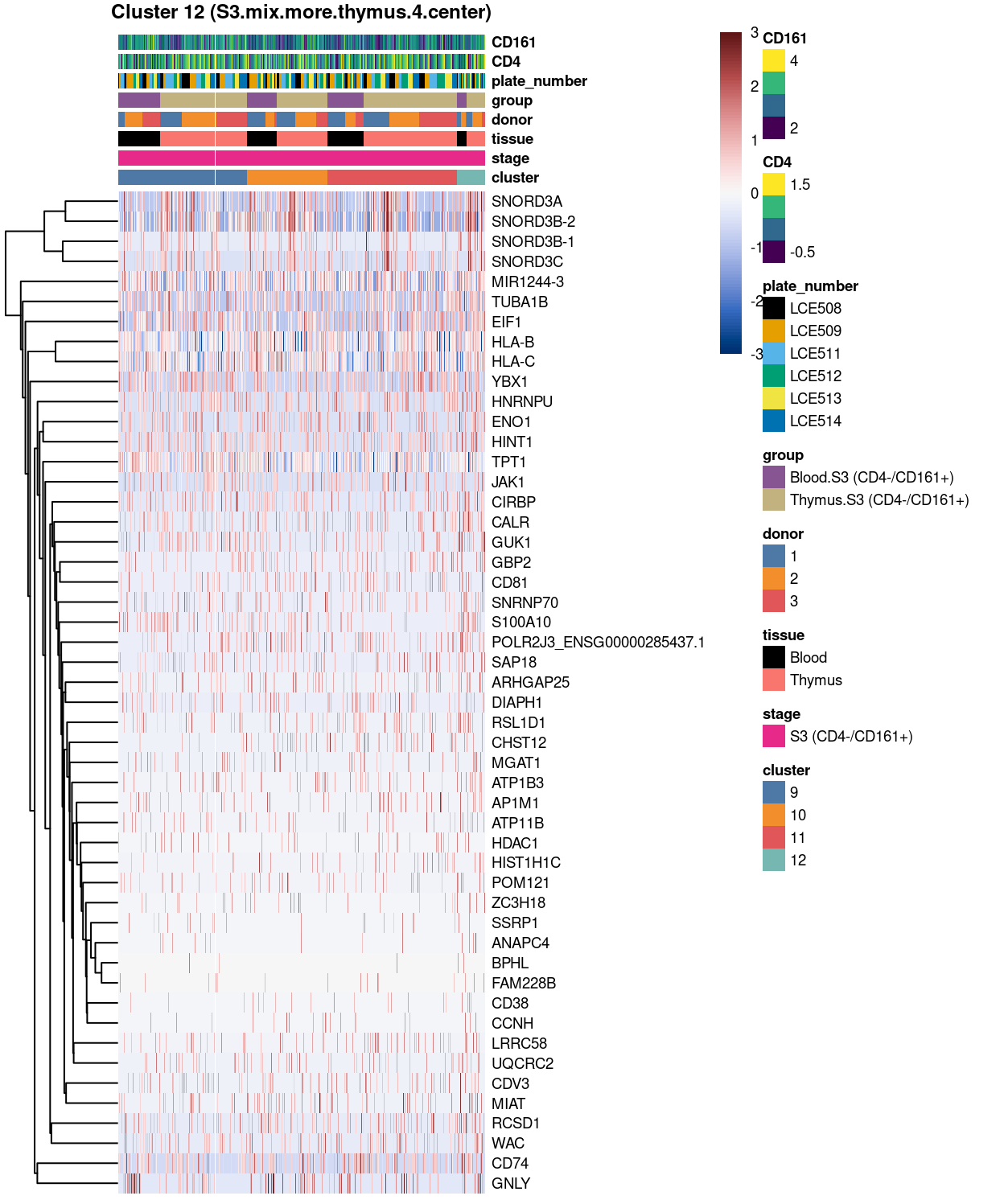
Figure 22: Heatmap of log-expression values in each sample for the top uniquely upregulated marker genes. Each column is a sample, each row a gene. Colours are capped at -3 and 3 to preserve dynamic range.

DGE lists of these comparisons are available in output/marker_genes/S3_only/uniquely_up/integrated/.

Summary: As in the minibulk with 20 DE only and we cannot tell the difference between thymus.s3 and blood.s3, there is no standout feature in terms of tissue-of-origin for each cluster of the “S3 only” subset and all of them are S3-mix (with mostly thymus.s3 blended with some blood.s3). Having said so, it may indicate that, S3 cells are somehow in common between thymus and blood, and based on gene expression difference, this subset of cells can be sub-divided into different sub-types.

By default parameter of the SNN algorithm, the “S3 only” subset contains six different clusters, but based on the UMAP, the clustering algorithm seems struggling, and based on my explorative analysis, four clusters is sufficient and can best demonstrate the heterogeneity of this subset dataset.

Based on the pairwise DE detection, each of the peripheral clusters (i.e. cluster 9, 10, 11) do have unique markers up-regulated and driving them apart.

For instance:

For cluster 9, the only global unique marker that can be found is IL7R, but when pairwise compare cluster 9 with the other clusters one by one, cluster 9 did show a number of gene feature that the other clusters do not have, such as gene LTB when compare 9 to 10, IFITM3, TOMM7 and S100A10 when compare 9 to 11, and lots of marker gene (such as CAPZA1, TPI1, and SLK) when compared 9 to 12.

Same applied to cluster 10, in which, the NPIPB gene family and the long non-coding RNA (AC009022.1) was shown as the global unique marker for cluster 10, then when pairwise compare cluster 9 with the other clusters one by one, cluster 10 did show a number of unique gene features, such as KLRD1 and CCL5 when compare 10 to 9, SYNE2 when compare 10 to 11, and series of markers (such as MBNL1 and RSF1) when compare 10 to 12.

For cluster 11, one can easily tell apart the cluster 9, 11, and 12, because CCL5 was up-regulated in cluster 11, but not cluster 9, whilst, a series of gene (such as MYO9B, SLK and CD1E) expressed in cluster 11, but not in 12. In contrast, we find no up-regulated markers when 11 to 10, but SYNE2, AC009022.1, and the NPIPB gene family when compare 10 to 11. All in all, cluster 11 is a separated cluster.

For cluster 12, no significantly up-regulated genes can be spotted when compare cluster 12 to all other 3 clusters. But as I shown you before, there are pack of genes significantly up-regulated in cluster 9, 10, and 11, but not in cluster 12. From the biological point of view, one possibility could be that the cluster 12 is a progenitor cell-type in the “S3 only” subset of the gamma-delta T cells, which could be multipotent and could be developed into either cluster 9, 10, or 11 cells depending on which set of markers it is going to express.

Supplemental info

Comparison of key marker expression by clusters

Show code

assay(sce, "log2cpm") <- edgeR::cpm(
  counts(sce),
  log = TRUE,
  lib.size = colSums(counts(sce)))

Show code

plot_grid(
  
  # cluster 9
  plotExpression(
    sce,
    features = "IL7R",
    x = "cluster",
    exprs_values = "log2cpm",
    colour_by = "cluster") +
    theme(axis.text.x = element_text(angle = 45, hjust = 1)) +
    scale_colour_manual(values = cluster_colours, name = "cluster"),
  
  plotExpression(
    sce,
    features = "LTB",
    x = "cluster",
    exprs_values = "log2cpm",
    colour_by = "cluster") +
    theme(axis.text.x = element_text(angle = 45, hjust = 1)) +
    scale_colour_manual(values = cluster_colours, name = "cluster"),
  
  plotExpression(
    sce,
    features = "IFITM3",
    x = "cluster",
    exprs_values = "log2cpm",
    colour_by = "cluster") +
    theme(axis.text.x = element_text(angle = 45, hjust = 1)) +
    scale_colour_manual(values = cluster_colours, name = "cluster"),

  plotExpression(
    sce,
    features = "TOMM7",
    x = "cluster",
    exprs_values = "log2cpm",
    colour_by = "cluster") +
    theme(axis.text.x = element_text(angle = 45, hjust = 1)) +
    scale_colour_manual(values = cluster_colours, name = "cluster"),

  plotExpression(
    sce,
    features = "S100A10",
    x = "cluster",
    exprs_values = "log2cpm",
    colour_by = "cluster") +
    theme(axis.text.x = element_text(angle = 45, hjust = 1)) +
    scale_colour_manual(values = cluster_colours, name = "cluster"),
      
  # cluster 10 and 11
  plotExpression(
    sce,
    features = "AC009022.1",
    x = "cluster",
    exprs_values = "log2cpm",
    colour_by = "cluster") +
    theme(axis.text.x = element_text(angle = 45, hjust = 1)) +
    scale_colour_manual(values = cluster_colours, name = "cluster"),
  
  plotExpression(
    sce,
    features = "SYNE2",
    x = "cluster",
    exprs_values = "log2cpm",
    colour_by = "cluster") +
    theme(axis.text.x = element_text(angle = 45, hjust = 1)) +
    scale_colour_manual(values = cluster_colours, name = "cluster"),

  plotExpression(
    sce,
    features = "KLRD1",
    x = "cluster",
    exprs_values = "log2cpm",
    colour_by = "cluster") +
    theme(axis.text.x = element_text(angle = 45, hjust = 1)) +
    scale_colour_manual(values = cluster_colours, name = "cluster"),
    
  plotExpression(
    sce,
    features = "CCL5",
    x = "cluster",
    exprs_values = "log2cpm",
    colour_by = "cluster") +
    theme(axis.text.x = element_text(angle = 45, hjust = 1)) +
    scale_colour_manual(values = cluster_colours, name = "cluster"),
    
  # cluster 12
  plotExpression(
    sce,
    features = "ACTG1",
    x = "cluster",
    exprs_values = "log2cpm",
    colour_by = "cluster") +
    theme(axis.text.x = element_text(angle = 45, hjust = 1)) +
    scale_colour_manual(values = cluster_colours, name = "cluster"),
  
  plotExpression(
    sce,
    features = "MBNL1",
    x = "cluster",
    exprs_values = "log2cpm",
    colour_by = "cluster") +
    theme(axis.text.x = element_text(angle = 45, hjust = 1)) +
    scale_colour_manual(values = cluster_colours, name = "cluster"),

  plotExpression(
    sce,
    features = "CAPZA1",
    x = "cluster",
    exprs_values = "log2cpm",
    colour_by = "cluster") +
    theme(axis.text.x = element_text(angle = 45, hjust = 1)) +
    scale_colour_manual(values = cluster_colours, name = "cluster"),

  plotExpression(
    sce,
    features = "SLK",
    x = "cluster",
    exprs_values = "log2cpm",
    colour_by = "cluster") +
    theme(axis.text.x = element_text(angle = 45, hjust = 1)) +
    scale_colour_manual(values = cluster_colours, name = "cluster"),

  plotExpression(
    sce,
    features = "CD1E",
    x = "cluster",
    exprs_values = "log2cpm",
    colour_by = "cluster") +
    theme(axis.text.x = element_text(angle = 45, hjust = 1)) +
    scale_colour_manual(values = cluster_colours, name = "cluster"),
        
  ncol = 2)

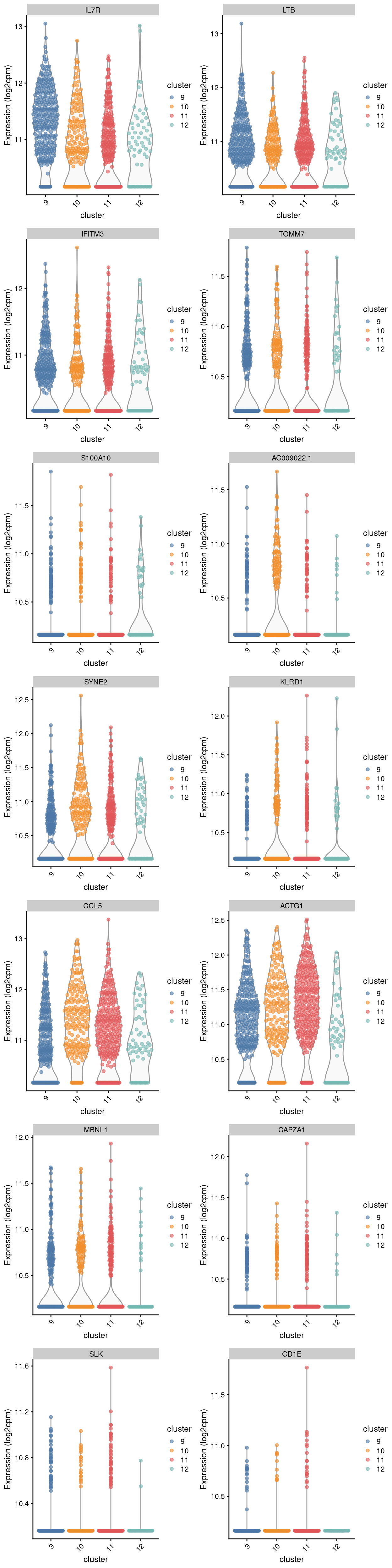
Figure 23: Violin plot showing the expression of key markers stratified by clusters

Expression of minibulk DE in the single-cell dataset

Show code

###############################################
# Heatmap using minibulk sig markers as feature

# laod package for read in csv.gz
library(data.table)
library(R.utils)

# read in
a <- fread(here("output", "DEGs", "excluding_blood_1-3", "Thymus.S3_vs_Blood.S3.aggregated_tech_reps.DEGs.csv.gz"))

# extract DEGlist (FDR < 0.05)
minibulkDEG.a <- a$ENSEMBL.GENENAME[a$FDR<0.05]

# divide the DE by UP and DOWN
minibulkDEG.a.up <- a$ENSEMBL.GENENAME[a$FDR<0.05 & a$logFC >0]
minibulkDEG.a.down <- a$ENSEMBL.GENENAME[a$FDR<0.05 & a$logFC <0]

# keep only unique markers
uniq.minibulkDEG.a <- Reduce(setdiff, list(minibulkDEG.a))
uniq.minibulkDEG.a.up <- Reduce(setdiff, list(minibulkDEG.a.up))
uniq.minibulkDEG.a.down <- Reduce(setdiff, list(minibulkDEG.a.down))

# check number of unique minibulkDEG in each
length(uniq.minibulkDEG.a)

[1] 20

Show code

length(uniq.minibulkDEG.a.up)

[1] 8

Show code

length(uniq.minibulkDEG.a.down)

[1] 12

Show code

# keep only top50
top.uniq.minibulkDEG.a <- if(length(uniq.minibulkDEG.a) >=50){uniq.minibulkDEG.a[1:50]} else {uniq.minibulkDEG.a}
minibulk_markers <- top.uniq.minibulkDEG.a

top.uniq.minibulkDEG.a.up <- if(length(uniq.minibulkDEG.a.up) >=50){uniq.minibulkDEG.a.up[1:50]} else {uniq.minibulkDEG.a.up}
minibulk_markers_up <- top.uniq.minibulkDEG.a.up

top.uniq.minibulkDEG.a.down <- if(length(uniq.minibulkDEG.a.down) >=50){uniq.minibulkDEG.a.down[1:50]} else {uniq.minibulkDEG.a.down}
minibulk_markers_down <- top.uniq.minibulkDEG.a.down

Show code

# NOTE: The following is a workaround to the lack of support for tabsets in 
#       distill (see https://github.com/rstudio/distill/issues/11 and 
#       https://github.com/rstudio/distill/issues/11#issuecomment-692142414 in 
#       particular).
xaringanExtra::use_panelset()

Minibulk DE_ALL_by cluster

Show code

library(scater)
plotHeatmap(
  sce,
  features = minibulk_markers,
  columns = order(
    sce$cluster,
    sce$stage,
    sce$tissue,
    sce$donor,
    sce$group,
    sce$plate_number),
  colour_columns_by = c(
    "cluster",
    "stage",
    "tissue",
    "donor",
    "group",
    "plate_number"),
  cluster_cols = FALSE,
  center = TRUE,
  symmetric = TRUE,
  zlim = c(-3, 3),
  show_colnames = FALSE,
  # TODO: temp trick to deal with the row-colouring problem
  annotation_row = data.frame(
    thymus.s3.vs.blood.s3 = factor(ifelse(minibulk_markers %in% top.uniq.minibulkDEG.a, "DE", "not DE"), levels = c("DE")),
    row.names = minibulk_markers),
  main = "Minibulk DE expression (UP and DOWN) in S3 subset (with cells divided by cluster)",
  column_annotation_colors = list(
    cluster = cluster_colours,
    stage = stage_colours,
    tissue = tissue_colours,
    donor = donor_colours,
    group = group_colours,
    plate_number = plate_number_colours),
  color = hcl.colors(101, "Blue-Red 3"),
  fontsize = 7)

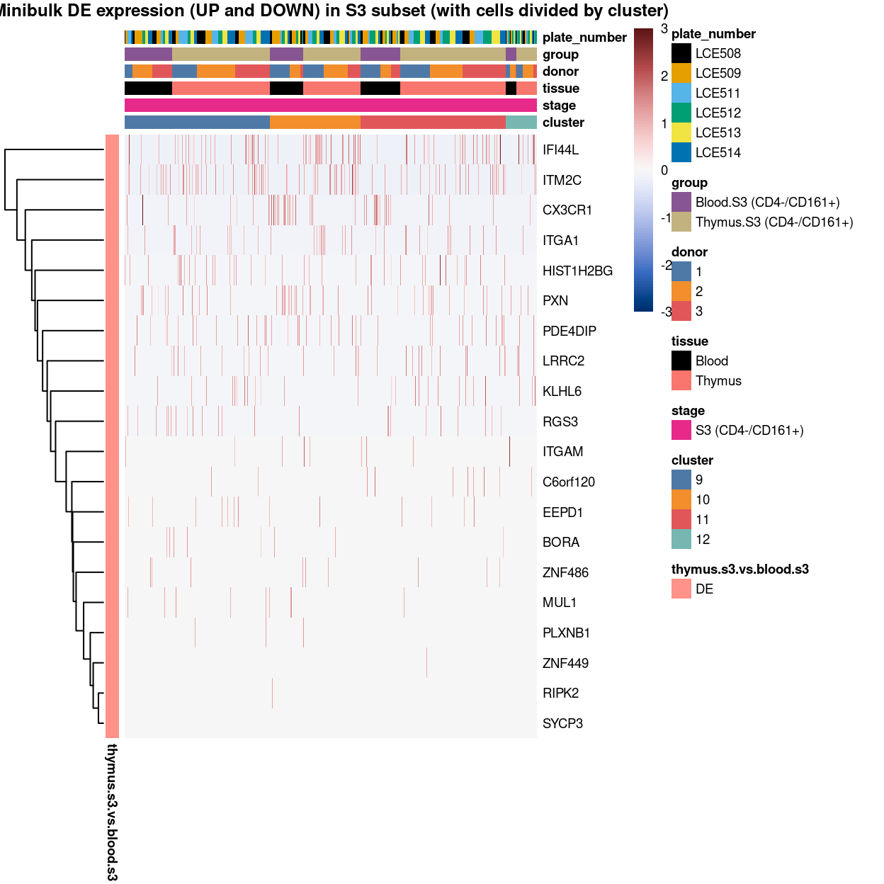
Figure 24: Heatmap of log-expression values in each sample for the marker genes identified from the mini-bulk analysis. Cells are ordered by cluster. Each column is a sample, each row a gene. Colours are capped at -3 and 3 to preserve dynamic range.

Minibulk DE_ALL_by group

Show code

library(scater)
plotHeatmap(
  sce,
  features = minibulk_markers,
  columns = order(
    sce$group,
    sce$stage,
    sce$tissue,
    sce$donor,
    sce$plate_number),
  colour_columns_by = c(
    "group",
    "stage",
    "tissue",
    "donor",
    "plate_number"),
  cluster_cols = FALSE,
  center = TRUE,
  symmetric = TRUE,
  zlim = c(-3, 3),
  show_colnames = FALSE,
  # TODO: temp trick to deal with the row-colouring problem
  annotation_row = data.frame(
    thymus.s3.vs.blood.s3 = factor(ifelse(minibulk_markers %in% top.uniq.minibulkDEG.a, "DE", "not DE"), levels = c("DE")),
    row.names = minibulk_markers),
  main = "Minibulk DE expression (UP and DOWN) in S3 subset (with cells divided by groups)",
  column_annotation_colors = list(
    group = group_colours,
    stage = stage_colours,
    tissue = tissue_colours,
    donor = donor_colours,
    plate_number = plate_number_colours),
  color = hcl.colors(101, "Blue-Red 3"),
  fontsize = 7)

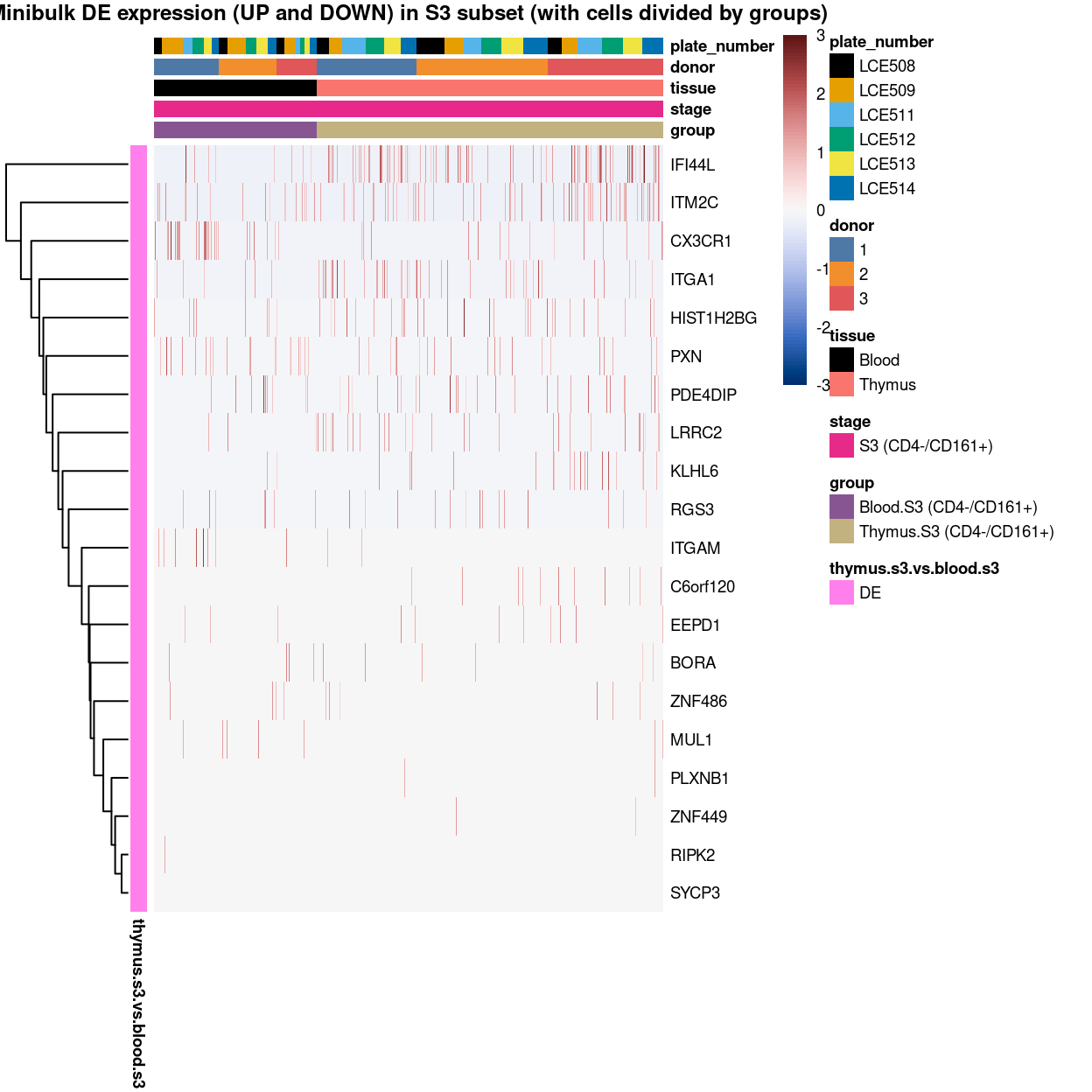
Figure 25: Heatmap of log-expression values in each sample for the marker genes identified from the mini-bulk analysis. Cells are ordered by group. Each column is a sample, each row a gene. Colours are capped at -3 and 3 to preserve dynamic range.

Minibulk DE_ALL_by group (clust_col)

Show code

library(scater)
plotHeatmap(
  sce,
  features = minibulk_markers,
  columns = order(
    sce$group,
    sce$stage,
    sce$tissue,
    sce$donor,
    sce$plate_number),
  colour_columns_by = c(
    "group",
    "stage",
    "tissue",
    "donor",
    "plate_number"),
  cluster_cols = TRUE,
  center = TRUE,
  symmetric = TRUE,
  zlim = c(-3, 3),
  show_colnames = FALSE,
  # TODO: temp trick to deal with the row-colouring problem
  annotation_row = data.frame(
    thymus.s3.vs.blood.s3 = factor(ifelse(minibulk_markers %in% top.uniq.minibulkDEG.a, "DE", "not DE"), levels = c("DE")),
    row.names = minibulk_markers),
  main = "Minibulk DE expression (UP and DOWN) in S3 subset (with cells divided by groups, column-clustered)",
  column_annotation_colors = list(
    group = group_colours,
    stage = stage_colours,
    tissue = tissue_colours,
    donor = donor_colours,
    plate_number = plate_number_colours),
  color = hcl.colors(101, "Blue-Red 3"),
  fontsize = 7)

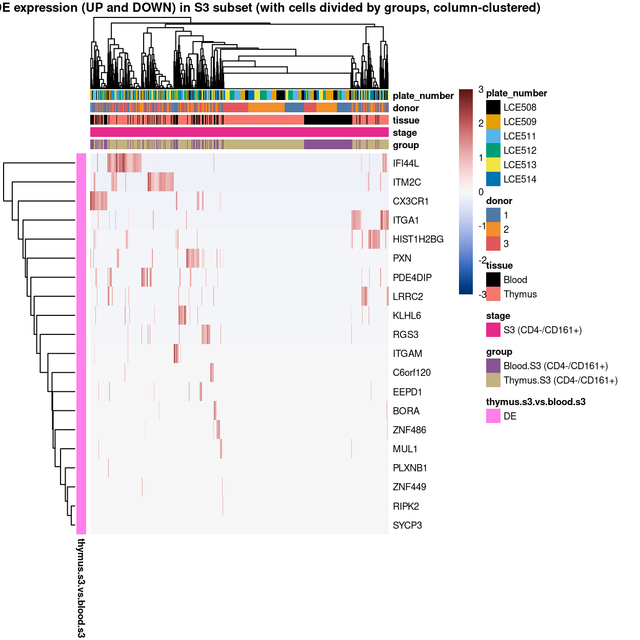
Figure 26: Heatmap of log-expression values in each sample for the marker genes identified from the mini-bulk analysis. Cells are ordered by group (column-clustered). Each column is a sample, each row a gene. Colours are capped at -3 and 3 to preserve dynamic range.

Minibulk DE_UP_by cluster

Show code

library(scater)
plotHeatmap(
  sce,
  features = minibulk_markers_up,
  columns = order(
    sce$cluster,
    sce$stage,
    sce$tissue,
    sce$donor,
    sce$group,
    sce$plate_number),
  colour_columns_by = c(
    "cluster",
    "stage",
    "tissue",
    "donor",
    "group",
    "plate_number"),
  cluster_cols = FALSE,
  center = TRUE,
  symmetric = TRUE,
  zlim = c(-3, 3),
  show_colnames = FALSE,
  # TODO: temp trick to deal with the row-colouring problem
  annotation_row = data.frame(
    thymus.s3.vs.blood.s3 = factor(ifelse(minibulk_markers_up %in% top.uniq.minibulkDEG.a, "DE", "not DE"), levels = c("DE")),
    row.names = minibulk_markers_up),
  main = "Minibulk DE expression (UP only) in S3 subset (with cells divided by clusters)",
  column_annotation_colors = list(
    cluster = cluster_colours,
    stage = stage_colours,
    tissue = tissue_colours,
    donor = donor_colours,
    group = group_colours,
    plate_number = plate_number_colours),
  color = hcl.colors(101, "Blue-Red 3"),
  fontsize = 7)

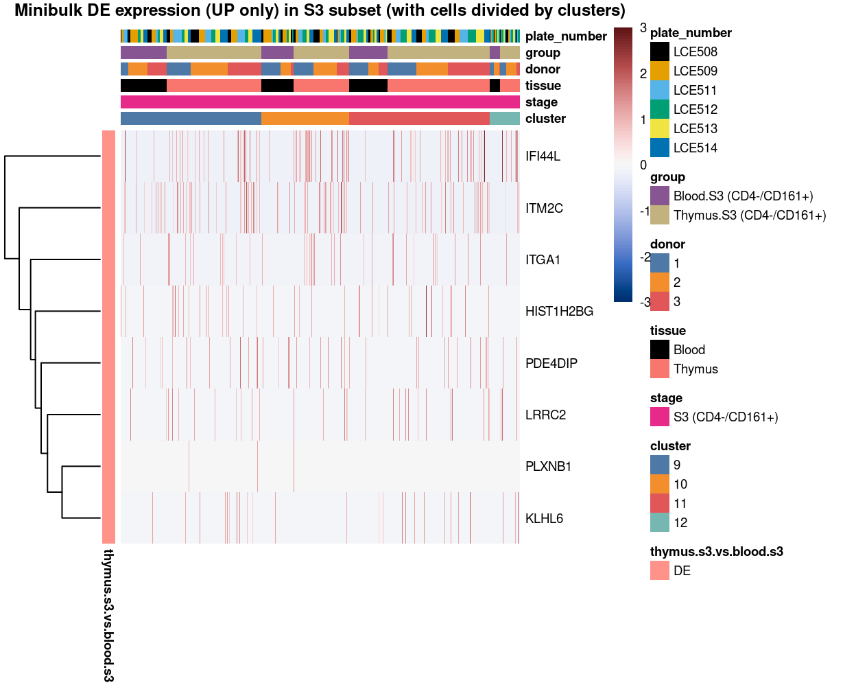
Figure 27: Heatmap of log-expression values in each sample for the marker genes (up-regulated) identified from the mini-bulk analysis. Cells are ordered by cluster. Each column is a sample, each row a gene. Colours are capped at -3 and 3 to preserve dynamic range.

Minibulk DE_UP_by group

Show code

library(scater)
plotHeatmap(
  sce,
  features = minibulk_markers_up,
  columns = order(
    sce$group,
    sce$stage,
    sce$tissue,
    sce$donor,
    sce$plate_number),
  colour_columns_by = c(
    "group",
    "stage",
    "tissue",
    "donor",
    "plate_number"),
  cluster_cols = FALSE,
  center = TRUE,
  symmetric = TRUE,
  zlim = c(-3, 3),
  show_colnames = FALSE,
  # TODO: temp trick to deal with the row-colouring problem
  annotation_row = data.frame(
    thymus.s3.vs.blood.s3 = factor(ifelse(minibulk_markers_up %in% top.uniq.minibulkDEG.a, "DE", "not DE"), levels = c("DE")),
    row.names = minibulk_markers_up),
  main = "Minibulk DE expression (UP only) in S3 subset (with cells divided by groups)",
  column_annotation_colors = list(
    group = group_colours,
    stage = stage_colours,
    tissue = tissue_colours,
    donor = donor_colours,
    plate_number = plate_number_colours),
  color = hcl.colors(101, "Blue-Red 3"),
  fontsize = 7)

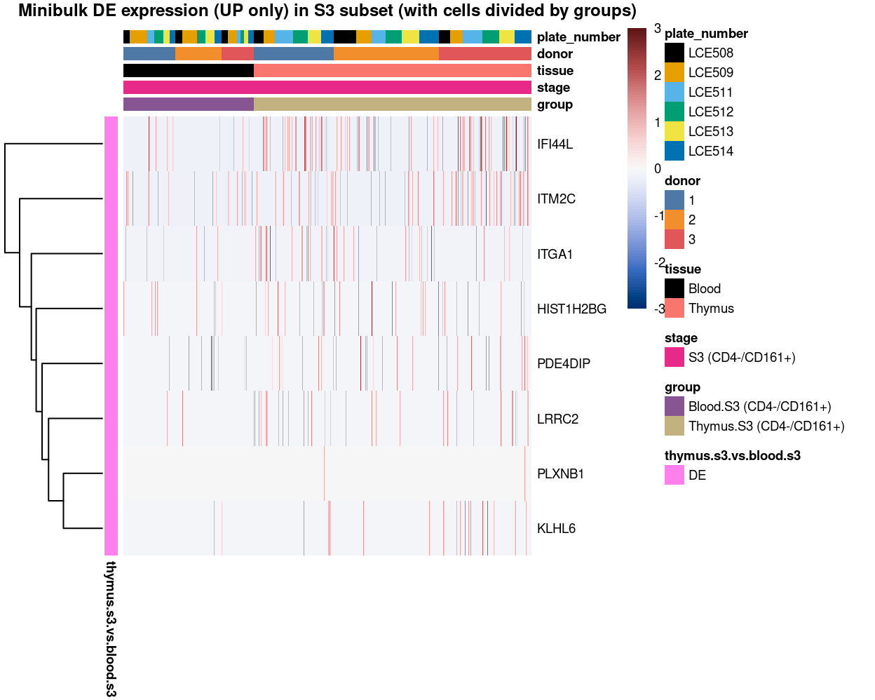
Figure 28: Heatmap of log-expression values in each sample for the marker genes (up-regulated) identified from the mini-bulk analysis. Cells are ordered by group. Each column is a sample, each row a gene. Colours are capped at -3 and 3 to preserve dynamic range.

Minibulk DE_UP_by group (clust_col)

Show code

library(scater)
plotHeatmap(
  sce,
  features = minibulk_markers_up,
  columns = order(
    sce$group,
    sce$stage,
    sce$tissue,
    sce$donor,
    sce$plate_number),
  colour_columns_by = c(
    "group",
    "stage",
    "tissue",
    "donor",
    "plate_number"),
  cluster_cols = TRUE,
  center = TRUE,
  symmetric = TRUE,
  zlim = c(-3, 3),
  show_colnames = FALSE,
  # TODO: temp trick to deal with the row-colouring problem
  annotation_row = data.frame(
    thymus.s3.vs.blood.s3 = factor(ifelse(minibulk_markers_up %in% top.uniq.minibulkDEG.a, "DE", "not DE"), levels = c("DE")),
    row.names = minibulk_markers_up),
  main = "Minibulk DE expression (UP only) in S3 subset (with cells divided by clusters, column-clustered)",
  column_annotation_colors = list(
    group = group_colours,
    stage = stage_colours,
    tissue = tissue_colours,
    donor = donor_colours,
    plate_number = plate_number_colours),
  color = hcl.colors(101, "Blue-Red 3"),
  fontsize = 7)

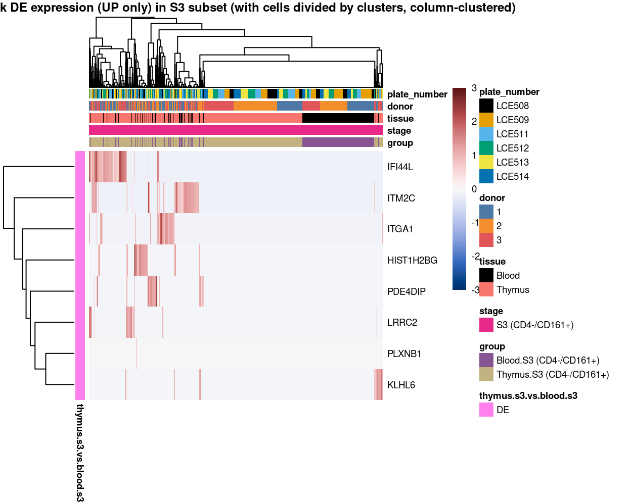
Figure 29: Heatmap of log-expression values in each sample for the marker genes (up-regulated) identified from the mini-bulk analysis. Cells are ordered by group (column-clustered). Each column is a sample, each row a gene. Colours are capped at -3 and 3 to preserve dynamic range.

Minibulk DE_DOWN_by cluster

Show code

library(scater)
plotHeatmap(
  sce,
  features = minibulk_markers_down,
  columns = order(
    sce$cluster,
    sce$stage,
    sce$tissue,
    sce$donor,
    sce$group,
    sce$plate_number),
  colour_columns_by = c(
    "cluster",
    "stage",
    "tissue",
    "donor",
    "group",
    "plate_number"),
  cluster_cols = FALSE,
  center = TRUE,
  symmetric = TRUE,
  zlim = c(-3, 3),
  show_colnames = FALSE,
  # TODO: temp trick to deal with the row-colouring problem
  annotation_row = data.frame(
    thymus.s3.vs.blood.s3 = factor(ifelse(minibulk_markers_down %in% top.uniq.minibulkDEG.a, "DE", "not DE"), levels = c("DE")),
    row.names = minibulk_markers_down),
  main = "Minibulk DE expression (DOWN only) in S3 subset (with cells divided by clusters)",
  column_annotation_colors = list(
    cluster = cluster_colours,
    stage = stage_colours,
    tissue = tissue_colours,
    donor = donor_colours,
    group = group_colours,
    plate_number = plate_number_colours),
  color = hcl.colors(101, "Blue-Red 3"),
  fontsize = 7)

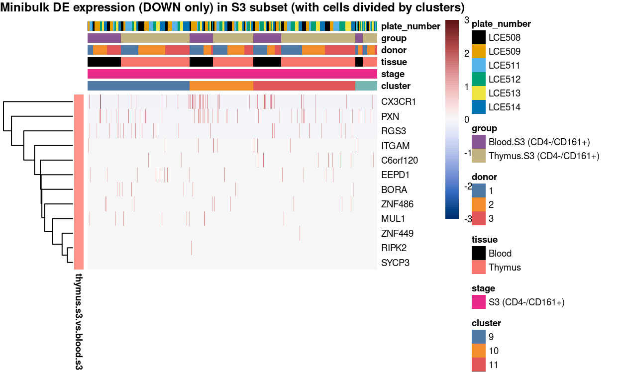
Figure 30: Heatmap of log-expression values in each sample for the marker genes (down-regulated) identified from the mini-bulk analysis. Cells are ordered by cluster. Each column is a sample, each row a gene. Colours are capped at -3 and 3 to preserve dynamic range.

Minibulk DE_DOWN_by group

Show code

library(scater)
plotHeatmap(
  sce,
  features = minibulk_markers_down,
  columns = order(
    sce$group,
    sce$stage,
    sce$tissue,
    sce$donor,
    sce$plate_number),
  colour_columns_by = c(
    "group",
    "stage",
    "tissue",
    "donor",
    "plate_number"),
  cluster_cols = FALSE,
  center = TRUE,
  symmetric = TRUE,
  zlim = c(-3, 3),
  show_colnames = FALSE,
  # TODO: temp trick to deal with the row-colouring problem
  annotation_row = data.frame(
    thymus.s3.vs.blood.s3 = factor(ifelse(minibulk_markers_down %in% top.uniq.minibulkDEG.a, "DE", "not DE"), levels = c("DE")),
    row.names = minibulk_markers_down),
  main = "Minibulk DE expression (DOWN only) in S3 subset (with cells divided by groups)",
  column_annotation_colors = list(
    grodown = group_colours,
    stage = stage_colours,
    tissue = tissue_colours,
    donor = donor_colours,
    plate_number = plate_number_colours),
  color = hcl.colors(101, "Blue-Red 3"),
  fontsize = 7)

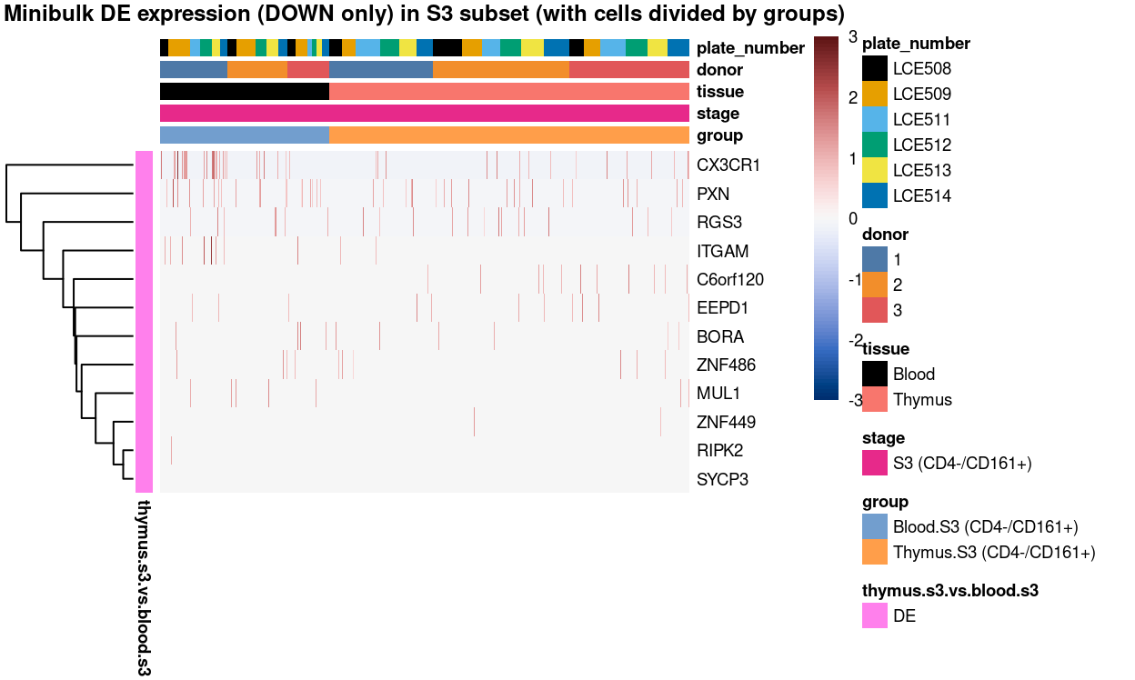
Figure 31: Heatmap of log-expression values in each sample for the marker genes (down-regulated) identified from the mini-bulk analysis. Cells are ordered by grodown. Each column is a sample, each row a gene. Colours are capped at -3 and 3 to preserve dynamic range.

Minibulk DE_DOWN_by group (clust_col)

Show code

library(scater)
plotHeatmap(
  sce,
  features = minibulk_markers_down,
  columns = order(
    sce$group,
    sce$stage,
    sce$tissue,
    sce$donor,
    sce$plate_number),
  colour_columns_by = c(
    "group",
    "stage",
    "tissue",
    "donor",
    "plate_number"),
  cluster_cols = TRUE,
  center = TRUE,
  symmetric = TRUE,
  zlim = c(-3, 3),
  show_colnames = FALSE,
  # TODO: temp trick to deal with the row-colouring problem
  annotation_row = data.frame(
    thymus.s3.vs.blood.s3 = factor(ifelse(minibulk_markers_down %in% top.uniq.minibulkDEG.a, "DE", "not DE"), levels = c("DE")),
    row.names = minibulk_markers_down),
  main = "Minibulk DE expression (DOWN only) in S3 subset (with cells divided by groups, column-clustered)",
  column_annotation_colors = list(
    grodown = group_colours,
    stage = stage_colours,
    tissue = tissue_colours,
    donor = donor_colours,
    plate_number = plate_number_colours),
  color = hcl.colors(101, "Blue-Red 3"),
  fontsize = 7)

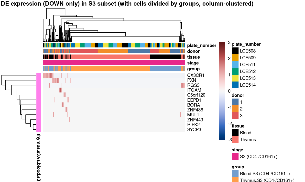
Figure 32: Heatmap of log-expression values in each sample for the marker genes (down-regulated) identified from the mini-bulk analysis. Cells are ordered by grodown (column-clustered). Each column is a sample, each row a gene. Colours are capped at -3 and 3 to preserve dynamic range.

Session info

The analysis and this document were prepared using the following software (click triangle to expand)

Show code

sessioninfo::session_info()

─ Session info ─────────────────────────────────────────────────────
 setting  value                       
 version  R version 4.0.5 (2021-03-31)
 os       CentOS Linux 7 (Core)       
 system   x86_64, linux-gnu           
 ui       X11                         
 language (EN)                        
 collate  en_US.UTF-8                 
 ctype    en_US.UTF-8                 
 tz       Australia/Melbourne         
 date     2023-03-28                  

─ Packages ─────────────────────────────────────────────────────────
 ! package              * version  date       lib
 P annotate               1.68.0   2020-10-27 [?]
 P AnnotationDbi          1.52.0   2020-10-27 [?]
 P assertthat             0.2.1    2019-03-21 [?]
 P batchelor            * 1.6.3    2021-04-16 [?]
 P beachmat               2.6.4    2020-12-20 [?]
 P beeswarm               0.3.1    2021-03-07 [?]
 P Biobase              * 2.50.0   2020-10-27 [?]
 P BiocGenerics         * 0.36.0   2020-10-27 [?]
 P BiocManager            1.30.12  2021-03-28 [?]
 P BiocNeighbors          1.8.2    2020-12-07 [?]
 P BiocParallel         * 1.24.1   2020-11-06 [?]
 P BiocSingular           1.6.0    2020-10-27 [?]
 P BiocStyle            * 2.18.1   2020-11-24 [?]
 P bit                    4.0.4    2020-08-04 [?]
 P bit64                  4.0.5    2020-08-30 [?]
 P bitops                 1.0-6    2013-08-17 [?]
 P blob                   1.2.1    2020-01-20 [?]
 P bluster                1.0.0    2020-10-27 [?]
 P bslib                  0.4.0    2022-07-16 [?]
 P cachem                 1.0.4    2021-02-13 [?]
 P cellranger             1.1.0    2016-07-27 [?]
 P cli                    2.4.0    2021-04-05 [?]
 P colorspace             2.0-0    2020-11-11 [?]
 P cowplot              * 1.1.1    2020-12-30 [?]
 P crayon                 1.4.1    2021-02-08 [?]
 P data.table           * 1.14.0   2021-02-21 [?]
 P DBI                    1.1.1    2021-01-15 [?]
 P DelayedArray           0.16.3   2021-03-24 [?]
 P DelayedMatrixStats     1.12.3   2021-02-03 [?]
 P DESeq2                 1.30.1   2021-02-19 [?]
 P digest                 0.6.27   2020-10-24 [?]
 P distill                1.2      2021-01-13 [?]
 P downlit                0.2.1    2020-11-04 [?]
 P dplyr                * 1.0.5    2021-03-05 [?]
 P dqrng                  0.2.1    2019-05-17 [?]
 P edgeR                * 3.32.1   2021-01-14 [?]
 P ellipsis               0.3.1    2020-05-15 [?]
 P evaluate               0.14     2019-05-28 [?]
 P fansi                  0.4.2    2021-01-15 [?]
 P farver                 2.1.0    2021-02-28 [?]
 P fastmap                1.1.0    2021-01-25 [?]
 P genefilter             1.72.1   2021-01-21 [?]
 P geneplotter            1.68.0   2020-10-27 [?]
 P generics               0.1.0    2020-10-31 [?]
 P GenomeInfoDb         * 1.26.4   2021-03-10 [?]
 P GenomeInfoDbData       1.2.4    2023-02-21 [?]
 P GenomicRanges        * 1.42.0   2020-10-27 [?]
 P ggbeeswarm             0.6.0    2017-08-07 [?]
 P ggplot2              * 3.3.3    2020-12-30 [?]
 P ggrepel              * 0.9.1    2021-01-15 [?]
 P Glimma               * 2.0.0    2020-10-27 [?]
 P glue                   1.4.2    2020-08-27 [?]
 P gridExtra              2.3      2017-09-09 [?]
 P gtable                 0.3.0    2019-03-25 [?]
 P here                 * 1.0.1    2020-12-13 [?]
 P highr                  0.9      2021-04-16 [?]
 P htmltools              0.5.3    2022-07-18 [?]
 P htmlwidgets            1.5.3    2020-12-10 [?]
 P httr                   1.4.2    2020-07-20 [?]
 P igraph                 1.2.6    2020-10-06 [?]
 P IRanges              * 2.24.1   2020-12-12 [?]
 P irlba                  2.3.3    2019-02-05 [?]
 P janitor              * 2.1.0    2021-01-05 [?]
 P jquerylib              0.1.3    2020-12-17 [?]
 P jsonlite               1.7.2    2020-12-09 [?]
 P knitr                  1.33     2021-04-24 [?]
 P labeling               0.4.2    2020-10-20 [?]
 P lattice                0.20-41  2020-04-02 [?]
 P lifecycle              1.0.0    2021-02-15 [?]
 P limma                * 3.46.0   2020-10-27 [?]
 P locfit                 1.5-9.4  2020-03-25 [?]
 P lubridate              1.7.10   2021-02-26 [?]
 P magrittr             * 2.0.1    2020-11-17 [?]
 P Matrix                 1.2-18   2019-11-27 [?]
 P MatrixGenerics       * 1.2.1    2021-01-30 [?]
 P matrixStats          * 0.58.0   2021-01-29 [?]
 P memoise                2.0.0    2021-01-26 [?]
 P msigdbr              * 7.2.1    2020-10-02 [?]
 P munsell                0.5.0    2018-06-12 [?]
 P patchwork            * 1.1.1    2020-12-17 [?]
 P pheatmap             * 1.0.12   2019-01-04 [?]
 P pillar                 1.5.1    2021-03-05 [?]
 P pkgconfig              2.0.3    2019-09-22 [?]
 P purrr                  0.3.4    2020-04-17 [?]
 P R.methodsS3          * 1.8.1    2020-08-26 [?]
 P R.oo                 * 1.24.0   2020-08-26 [?]
 P R.utils              * 2.10.1   2020-08-26 [?]
 P R6                     2.5.0    2020-10-28 [?]
 P RColorBrewer           1.1-2    2014-12-07 [?]
 P Rcpp                   1.0.6    2021-01-15 [?]
 P RCurl                  1.98-1.3 2021-03-16 [?]
 P readxl               * 1.3.1    2019-03-13 [?]
 P ResidualMatrix         1.0.0    2020-10-27 [?]
 P rlang                  0.4.11   2021-04-30 [?]
 P rmarkdown            * 2.14     2022-04-25 [?]
 P rprojroot              2.0.2    2020-11-15 [?]
 P RSQLite                2.2.5    2021-03-27 [?]
 P rsvd                   1.0.3    2020-02-17 [?]
 P S4Vectors            * 0.28.1   2020-12-09 [?]
 P sass                   0.4.2    2022-07-16 [?]
 P scales                 1.1.1    2020-05-11 [?]
 P scater               * 1.18.6   2021-02-26 [?]
 P scran                * 1.18.5   2021-02-04 [?]
 P scuttle                1.0.4    2020-12-17 [?]
 P sessioninfo            1.1.1    2018-11-05 [?]
 P SingleCellExperiment * 1.12.0   2020-10-27 [?]
 P snakecase              0.11.0   2019-05-25 [?]
 P sparseMatrixStats      1.2.1    2021-02-02 [?]
 P statmod                1.4.35   2020-10-19 [?]
 P stringi                1.7.3    2021-07-16 [?]
 P stringr                1.4.0    2019-02-10 [?]
 P SummarizedExperiment * 1.20.0   2020-10-27 [?]
 P survival               3.2-7    2020-09-28 [?]
 P tibble                 3.1.0    2021-02-25 [?]
 P tidyr                * 1.1.3    2021-03-03 [?]
 P tidyselect             1.1.0    2020-05-11 [?]
 P utf8                   1.2.1    2021-03-12 [?]
 P vctrs                  0.3.7    2021-03-29 [?]
 P vipor                  0.4.5    2017-03-22 [?]
 P viridis                0.5.1    2018-03-29 [?]
 P viridisLite            0.3.0    2018-02-01 [?]
 P withr                  2.4.1    2021-01-26 [?]
 P xaringanExtra          0.5.4    2023-02-21 [?]
 P xfun                   0.31     2022-05-10 [?]
 P XML                    3.99-0.6 2021-03-16 [?]
 P xtable                 1.8-4    2019-04-21 [?]
 P XVector                0.30.0   2020-10-27 [?]
 P yaml                   2.2.1    2020-02-01 [?]
 P zlibbioc               1.36.0   2020-10-27 [?]
 source                                  
 Bioconductor                            
 Bioconductor                            
 CRAN (R 4.0.5)                          
 Bioconductor                            
 Bioconductor                            
 CRAN (R 4.0.5)                          
 Bioconductor                            
 Bioconductor                            
 CRAN (R 4.0.5)                          
 Bioconductor                            
 Bioconductor                            
 Bioconductor                            
 Bioconductor                            
 CRAN (R 4.0.5)                          
 CRAN (R 4.0.5)                          
 CRAN (R 4.0.5)                          
 CRAN (R 4.0.5)                          
 Bioconductor                            
 CRAN (R 4.0.5)                          
 CRAN (R 4.0.5)                          
 CRAN (R 4.0.5)                          
 CRAN (R 4.0.5)                          
 CRAN (R 4.0.5)                          
 CRAN (R 4.0.5)                          
 CRAN (R 4.0.5)                          
 CRAN (R 4.0.5)                          
 CRAN (R 4.0.5)                          
 Bioconductor                            
 Bioconductor                            
 Bioconductor                            
 CRAN (R 4.0.5)                          
 CRAN (R 4.0.5)                          
 CRAN (R 4.0.5)                          
 CRAN (R 4.0.5)                          
 CRAN (R 4.0.5)                          
 Bioconductor                            
 CRAN (R 4.0.5)                          
 CRAN (R 4.0.5)                          
 CRAN (R 4.0.5)                          
 CRAN (R 4.0.5)                          
 CRAN (R 4.0.5)                          
 Bioconductor                            
 Bioconductor                            
 CRAN (R 4.0.5)                          
 Bioconductor                            
 Bioconductor                            
 Bioconductor                            
 CRAN (R 4.0.5)                          
 CRAN (R 4.0.5)                          
 CRAN (R 4.0.5)                          
 Bioconductor                            
 CRAN (R 4.0.5)                          
 CRAN (R 4.0.5)                          
 CRAN (R 4.0.5)                          
 CRAN (R 4.0.5)                          
 CRAN (R 4.0.5)                          
 CRAN (R 4.0.5)                          
 CRAN (R 4.0.5)                          
 CRAN (R 4.0.5)                          
 CRAN (R 4.0.5)                          
 Bioconductor                            
 CRAN (R 4.0.5)                          
 CRAN (R 4.0.5)                          
 CRAN (R 4.0.5)                          
 CRAN (R 4.0.5)                          
 CRAN (R 4.0.5)                          
 CRAN (R 4.0.5)                          
 CRAN (R 4.0.3)                          
 CRAN (R 4.0.5)                          
 Bioconductor                            
 CRAN (R 4.0.5)                          
 CRAN (R 4.0.5)                          
 CRAN (R 4.0.5)                          
 CRAN (R 4.0.3)                          
 Bioconductor                            
 CRAN (R 4.0.5)                          
 CRAN (R 4.0.5)                          
 CRAN (R 4.0.5)                          
 CRAN (R 4.0.5)                          
 CRAN (R 4.0.5)                          
 CRAN (R 4.0.5)                          
 CRAN (R 4.0.5)                          
 CRAN (R 4.0.5)                          
 CRAN (R 4.0.5)                          
 CRAN (R 4.0.5)                          
 CRAN (R 4.0.5)                          
 CRAN (R 4.0.5)                          
 CRAN (R 4.0.5)                          
 CRAN (R 4.0.5)                          
 CRAN (R 4.0.5)                          
 CRAN (R 4.0.5)                          
 CRAN (R 4.0.5)                          
 Bioconductor                            
 CRAN (R 4.0.5)                          
 CRAN (R 4.0.5)                          
 CRAN (R 4.0.5)                          
 CRAN (R 4.0.5)                          
 CRAN (R 4.0.5)                          
 Bioconductor                            
 CRAN (R 4.0.5)                          
 CRAN (R 4.0.5)                          
 Bioconductor                            
 Bioconductor                            
 Bioconductor                            
 CRAN (R 4.0.5)                          
 Bioconductor                            
 CRAN (R 4.0.5)                          
 Bioconductor                            
 CRAN (R 4.0.5)                          
 CRAN (R 4.0.5)                          
 CRAN (R 4.0.5)                          
 Bioconductor                            
 CRAN (R 4.0.3)                          
 CRAN (R 4.0.5)                          
 CRAN (R 4.0.5)                          
 CRAN (R 4.0.5)                          
 CRAN (R 4.0.5)                          
 CRAN (R 4.0.5)                          
 CRAN (R 4.0.5)                          
 CRAN (R 4.0.5)                          
 CRAN (R 4.0.5)                          
 CRAN (R 4.0.5)                          
 Github (gadenbuie/xaringanExtra@5e2d80b)
 CRAN (R 4.0.5)                          
 CRAN (R 4.0.5)                          
 CRAN (R 4.0.5)                          
 Bioconductor                            
 CRAN (R 4.0.5)                          
 Bioconductor                            

[1] /stornext/Projects/score/Analyses/C094_Pellicci/renv/library/R-4.0/x86_64-pc-linux-gnu
[2] /stornext/System/data/apps/R/R-4.0.5/lib64/R/library

 P ── Loaded and on-disk path mismatch.

---

1. Differential expression analyses is performed on the original log-expression values. We do not use the MNN-corrected values here except to obtain the clusters to be characterized.↩︎